RF-controlled robot design requires S parameters to model and simulate various electronic passive resistors, inductors, and capacitor circuits represented as two-port networks.
Examples demonstrating the usefulness of the technique and models in simulation are provided.
The procedure and technique for simulation of two ports using Z, H parameters are extended by similar steps using analogue behavioural modelling, as is done for S parameters in a two-port with original SPICE2G for robotic circuits, using computer-aided simulation tools like SPICE/ Pspice at high frequencies.

Introduction
In the present age of modern electronics, almost all engineers and scientists are familiar with robots as they are extensively used in human life.
The RF-controlled Robot utilises a transmitting device containing an RF transmitter and an RF Encoder, sending commands to the robots for specified tasks such as moving back and forth, reversing, turning right/left, and stopping.
To design RF transmitters in RF and microwave systems, S-parameters [1-6] are common, and these parameters can be measured with the help of network analysers.
SPICE [7-16] is employed to simulate various electronic circuits comprising different types of devices and linear circuits.
The elements used in typical CAD device environments using SPICE include resistors, capacitors, inductors (including mutual), voltage/current DC and AC sources, dependent linear and non-linear current/voltage sources, transmission lines, and electronic devices such as diodes, BJT, JFET, MOSFET.
Two-port circuit models for microwave passive networks, both in classroom theory and industrial practice, are important for students and researchers and are useful in synthesising T-PI models [17-24].
There are two methods to simulate [18-24] active or passive circuits: the first is by using active or passive models for each component or group of components, and the second is by representing input and output voltages and currents by suitable port parameter equations when that portion of the circuit does not contain independent voltage and current sources.
Models represented by non-linear analogue behavioural options of Pspice are added to these equations, and the system is solved for voltages and currents, either manually or using sophisticated simulation software.
To model the two-port of an RF network for robotic use using existing software programs like Spice2g and Pspice, where there are no models to represent them, we must use existing model descriptions like behavioural models and adapt them suitably.
Attempts have been made to achieve this using only the Spice2G program. The present method can be used in conjunction with original passive circuits to simulate networks.
The analogue behavioural modelling option of PSPICE includes additional descriptions of DC and AC voltages and currents using expressions, tables, Laplacian operators, and complex voltage and current multiplications with complex numbers.
Passive Circuit Modelling Method
The power waves incident and reflected from the two ports of a linear network are defined as a1, a2, b1, and b2, respectively. These are related to the scattering matrix that characterises the circuit.
b1=S11a1+S12a2
b2=S21a1+S22a2 (1)
where,
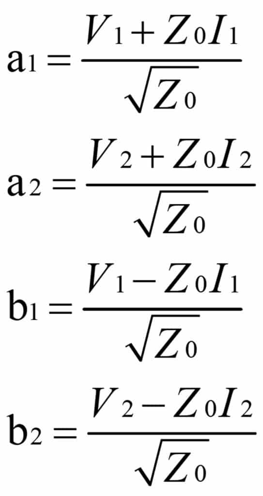
Here, both ports are assumed to have the same characteristic impedance Z0. Substituting for a1, a2, b1, b2 in equation (1),
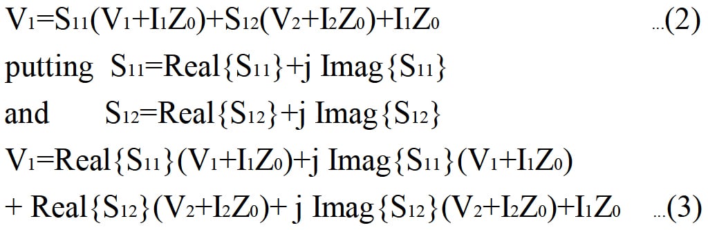
Similarly,
V2=S22(V2+I2Z0)+S21(V1+I1Z0)+I2Z0 …(4)
putting S22=Real{S22}+ j Imag{S22}
and S21=Real{S21}+ j Imag{S21} …(5)
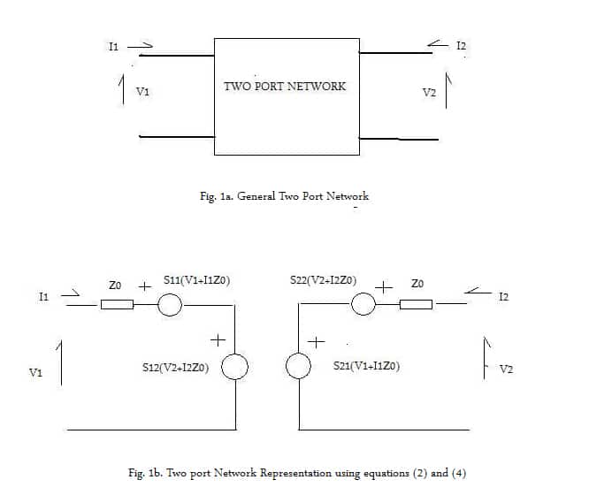
Now, equation (2) and (4) describing the two port voltages and currents (Fig.1a) could be represented by Fig. 1b. Now,
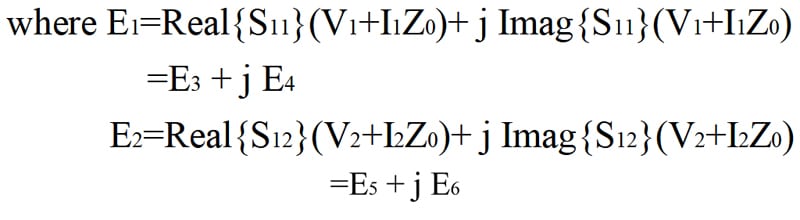
V1 i.e., equation(3) can be written as V1=I1Z0+E1+E2
V2 i.e, equation (5) can be written as V2=I2Z0+E7+E8
where E7=Real{S22}(V2+I2Z0)+ j Imag{S22}(V2+I2Z0)
=E9+j E10
E8=Real{S21}(V1+I1Z0)+ j Imag{S21}(V1+I1Z0)
=E11+j E12
If the S parameters are defined in rectangular(Cartesian) co-ordinates, i.e., Sij=Real{Sij}+jImag{Sij}, i,j (1,2) the sub-circuit in Table I should be used for simulating two-port network between terminals 1 and 2.
If the S parameters are defined in polar coordinates, the Table II sub circuits should be used for defining two-port networks.
If SPICE2G version is used, a lossless transmission line of length NL chosen according to Polar angles of the S parameters is used to realise the e jPhase Angle term.
If the phase angle is negative NL(Spice transmission line parameter) is given by
![]() =ANG1
=ANG1
And if Phase Angle is positive then NL is given by
![]() =ANG2
=ANG2
Results
The overall S parameters of the entire circuit (Figure 2) which is used generally in radio transmitters to control robots, are computed by PSpice files.
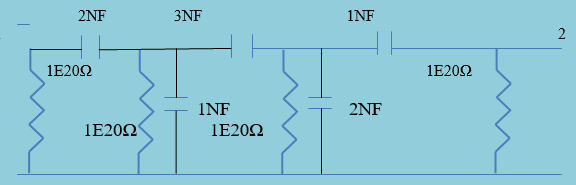
A two-port model for the measured S parameters for the radio frequency transmitter component (FIGURE 2) with S11, S21, S12, and S22 as inputs is obtained USING BOTH SPICE2G and Pspice circuit analyses and simulation software.
Analog behavioural modelling technique is used with Pspice. Table I and Table II show the SPICE2G subroutines to obtain any two port equivalent using scattering matrix for radio frequency transmitter component for robot control.
Table I: SPICE2G file model for Simulating Two Port with Cartesian S Parameters
| .SUBCKT MODEL1 1 2 |
| E3 10 0 POLY(2) 1 0 3 4 0 ReS11 ReS11 |
| E4 20 0 POLY(2) 1 0 3 4 0 ImS11 ImS11 |
| V13 1 3 AC 0 |
| R34 3 4 50 |
| *where Real{S11}=ReS11 and Imag{S11}=ImS11 |
| *The following description gets jE4 |
| E210 21 0 20 0 1 |
| V22 22 0 AC 0 |
| *CURRENT THROUGH CAPACITANCE C2122 = j ωC2122 E210 where ω is angular *frequency |
| *AT THE GIVEN S PARAMETER FREQUENCY CHOOSING ωC2122=1 OR C2122=1/ω |
| C2122 21 22 1/ω |
| *CONVERT THE CURRENT INTO VOLTAGE BY CURRENT CONTROLLED |
| *CURRENT GENERATOR F230 |
| F230 0 23 V22 1 |
| R230 23 0 1 |
| E1 4 5 POLY(2) 10 0 23 0 0 1 1 |
| E5 11 0 POLY(2) 2 0 6 7 0 ReS12 ReS12 |
| E6 12 0 POLY(2) 2 0 6 7 0 ImS12 ImS12 |
| *where Real{S12}=ReS12 and Imag{S12}=ImS12 |
| *TO GET jE6 |
| E240 24 0 12 0 1 |
| V25 25 0 AC 0 |
| *CURRENT THROUGH CAPACITANCE C2425=j ωC2425 E240 where ω is angular *frequency |
| *AT THE GIVEN S PARAMETER FREQUENCY CHOOSING ωC2425=1 OR C2425=1/ω |
| C2425 24 25 1/ω |
| *CONVERT THE CURRENT INTO VOLTAGE BY CURRENT CONTROLLED |
| *CURRENT GENERATOR F260 |
| F260 0 26 V25 1 |
| R260 26 0 1 |
| E2 5 0 POLY(2) 11 0 26 0 0 1 1 |
| E9 30 0 POLY(2) 2 0 6 7 0 ReS22 ReS22 |
| E10 40 0 POLY(2) 2 0 6 7 0 ImS22 ImS22 |
| R67 6 7 50 |
| V26 2 6 AC 0 |
| *where Real{S22}=ReS22 and Imag{S22}=ImS22 |
| *TO GET jE10 |
| E310 31 0 40 0 1 |
| V32 32 0 AC 0 |
| *CURRENT THROUGH CAPACITANCE C3132 = j ωC3132 E310 where ω is angular *frequency |
| *AT THE GIVEN S PARAMETER FREQUENCY CHOOSING ωC3132=1 OR C3132=1/ω |
| C3132 31 32 1/ω |
| *CONVERT THE CURRENT INTO VOLTAGE BY CURRENT CONTROLLED |
| *CURRENT GENERATOR F330 |
| F330 0 33 V32 1 |
| R330 33 0 1 |
| E7 7 8 POLY(2) 30 0 33 0 0 1 1 |
| E11 41 0 POLY(2) 1 0 3 4 0 ReS21 ReS21 |
| E12 42 0 POLY(2) 1 0 3 4 0 21 ImS21 ImS21 |
| *where Real{S21}=ReS21 and Imag{S21}=ImS21 |
| *TO GET jE12 |
| E430 43 0 42 0 1 |
| V44 44 0 AC 0 |
| *CURRENT THROUGH CAPACITANCE C4344 = j ωC4344 E430 where ω is angular *frequency |
| *AT THE GIVEN S PARAMETER FREQUENCY CHOOSING ωC4344=1 OR C4344=1/ω |
| C4344 43 44 1/ω |
| *CONVERT THE CURRENT INTO VOLTAGE BY CURRENT CONTROLLED |
| *CURRENT GENERATOR F450 |
| F450 0 45 V44 1 |
| R450 45 0 1 |
| E8 8 0 POLY(2) 41 0 45 0 0 1 1 |
| .ENDS MODEL1 |
Table II: SPICE2G file model to simulate Two ports with Polar S parameters
| .SUBCKT MODEL2 1 2 |
| *S11M is the magnitude of the S11 of the two port |
| *F0 is the frequency at which S parameters are defined |
| E3 10 0 POLY(2) 1 0 3 4 0 S11M S11M |
| T1 10 0 11 0 Z0=50 F= F0 NL=ANG1 or ANG2 for S11 Phase |
| RZ0 11 0 50 |
| *S12M is the magnitude of the S12 of the two port |
| E4 12 0 POLY(2) 2 0 6 7 0 S12M S12M |
| T2 12 0 13 0 Z0=50 F= F0 NL=ANG1 or ANG2 for S12 Phase |
| R130Z0 13 0 50 |
| *PORT 1 DESCRIPTION |
| V13 1 3 AC 0 |
| R34 3 4 50 |
| E1 4 5 11 0 1 |
| E2 5 0 13 0 1 |
| *S22M is the magnitude of the S22 of the two port |
| E5 20 0 POLY(2) 2 0 6 7 0 S22M S22M |
| T3 20 0 21 0 Z0=50 F = F0 NL=ANG1 or ANG2 for S22 Phase |
| R210Z0 21 0 50 |
| *S21M is the magnitude of the S21 of the two port |
| E6 30 0 POLY(2) 1 0 3 4 0 S21M S21M |
| T4 30 0 31 0 Z0=50 F= F0 NL= ANG1 or ANG2 for S21 Phase |
| R310Z0 31 0 50 |
| *PORT 2 DESCRIPTION |
| V26 2 6 AC 0 |
| R67 6 7 50 |
| E7 7 8 21 0 1 |
| E8 8 0 31 0 1 |
| .ENDS MODEL2 |
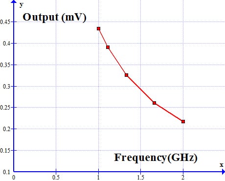
Tables III and IV show the circuit netlist to obtain S parameters for Figure 2. Table V shows the equivalent two-port circuit for Figure 2. with Pspice software. Figures 3a & 3b show the output voltage of the transmitter component with 100Ω source and load.
Table III: Netlist for S parameter determination S11, S21
| **** 08/18/23 16:25:38 ****** PSpice Lite (October 2012) ****** ID# 10813 **** |
| S parameters of capacitive passive circuit |
| ************************************************************************ |
| C13 1 3 2NF |
| C30 3 0 1NF |
| C34 3 4 3NF |
| C40 4 0 2NF |
| C42 4 2 1NF |
| R20 2 0 1E24 |
| R40 4 0 1E24 |
| R30 3 0 1E24 |
| R10 1 0 1E24 |
| R15 1 5 50 |
| V10 5 0 AC 1 |
| R220 2 0 50 |
| E1 6 0 VALUE={2*V(1)-V(7)} |
| R60 6 0 1 |
| V70 7 0 AC 1 |
| R70 7 0 1 |
| E2 8 0 2 0 2 |
| R80 8 0 1 |
| .AC LIN 10 1GHZ 10GHZ |
| *VOLTAGE AT NODE (8) GIVES S21 |
| *VOLTAGE AT NODE (6) GIVES S11 |
| .PRINT AC VM(8) VP(8) VM(6) VP(6) |
| .PRINT AC IM(V10) IP(V10) |
| .END |
| **** 08/18/23 16:25:38 ****** PSpice Lite (October 2012) ****** ID# 10813 **** |
| S parameters of capacitive passive circuit |
| **** 08/18/23 16:25:38 ****** PSpice Lite (October 2012) ****** ID# 10813 **** |
| S parameters of capacitive passive circuit |
| **** AC analysis Temperature = 27.000 DEG C |
| ************************************************************************ |
| FREQ VM(8) VP(8) VM(6) VP(6) |
| 1.000E+09 1.736E-03 -8.958E+01 1.000E+00 -1.797E+02 |
| 2.000E+09 8.681E-04 -8.979E+01 1.000E+00 -1.798E+02 |
| 3.000E+09 5.787E-04 -8.986E+01 1.000E+00 -1.799E+02 |
| 4.000E+09 4.341E-04 -8.989E+01 1.000E+00 -1.799E+02 |
| 5.000E+09 3.472E-04 -8.992E+01 1.000E+00 -1.799E+02 |
| 6.000E+09 2.894E-04 -8.993E+01 1.000E+00 -1.799E+02 |
| 7.000E+09 2.480E-04 -8.994E+01 1.000E+00 -1.800E+02 |
| 8.000E+09 2.170E-04 -8.995E+01 1.000E+00 -1.800E+02 |
| 9.000E+09 1.929E-04 -8.995E+01 1.000E+00 -1.800E+02 |
| 1.000E+10 1.736E-04 -8.996E+01 1.000E+00 -1.800E+02 |
Table IV: Netlist for S parameter determination S12, S22
| **** 08/18/23 16:36:51 ****** PSpice Lite (October 2012) ****** ID# 10813 **** |
| S parameters of capacitive passive (FILE2) |
| ****************************************************************************** |
| C13 1 3 2NF |
| C30 3 0 1NF |
| C34 3 4 3NF |
| C40 4 0 2NF |
| C42 4 2 1NF |
| R20 2 0 1E24 |
| R40 4 0 1E24 |
| R30 3 0 1E24 |
| R10 1 0 1E24 |
| R15 2 5 50 |
| V10 5 0 AC 1 |
| R220 1 0 50 |
| E1 6 0 VALUE={2*V(2)-V(7)} |
| R60 6 0 1 |
| V70 7 0 AC 1 |
| R70 7 0 1 |
| E2 8 0 1 0 2 |
| R80 8 0 1 |
| *VOLTAGE AT NODE (6) GIVES S22 |
| *VOLTAGE AT NODE (8) GIVES S12 |
| .AC LIN 10 1GHZ 10GHZ |
| .PRINT AC VM(8) VP(8) VM(6) VP(6) |
| .END |
| S parameters of capacitive passive (FILE2) |
| TOTAL POWER DISSIPATION 0.00E+00 WATTS |
| S parameters of capacitive passive (FILE2) |
| **** AC analysis Temperature = 27.000 DEG C |
| ****************************************************************************** |
| FREQ VM(8) VP(8) VM(6) VP(6) |
| 1.000E+09 1.736E-03 -8.958E+01 1.000E+00 -1.795E+02 |
| 2.000E+09 8.681E-04 -8.979E+01 1.000E+00 -1.798E+02 |
| 3.000E+09 5.787E-04 -8.986E+01 1.000E+00 -1.798E+02 |
| 4.000E+09 4.341E-04 -8.989E+01 1.000E+00 -1.799E+02 |
| 5.000E+09 3.472E-04 -8.992E+01 1.000E+00 -1.799E+02 |
| 6.000E+09 2.894E-04 -8.993E+01 1.000E+00 -1.799E+02 |
| 7.000E+09 2.480E-04 -8.994E+01 1.000E+00 -1.799E+02 |
| 8.000E+09 2.170E-04 -8.995E+01 1.000E+00 -1.799E+02 |
| 9.000E+09 1.929E-04 -8.995E+01 1.000E+00 -1.799E+02 |
| 1.000E+10 1.736E-04 -8.996E+01 1.000E+00 -1.800E+02 |
| Job concluded |
The results by running the file(Table V) show that the two port representations are correct and valid in the 1Ghz, and 2GHz and verified by Tables III and IV.
Table V: Two-port representation of the Transmitter Control Circuit
| **** 08/18/23 16:49:19 ****** PSpice Lite (October 2012) ****** ID# 10813 **** |
| Capacitive passive circuit equivalent simulation |
| **** Circuit description |
| **************************************************************************** |
| V50 9 0 AC 1 |
| V93 9 3 |
| R31 3 1 50 |
| R12 1 11 50 |
| E1 11 4 FREQ {V(1)+I(V93)*50}=(1GHZ, 0.,-179.7) (2GHZ,0.,-179.8) |
| E2 4 0 FREQ {V(2)+I(V27)*50}=(1GHZ,-55.209,-89.58) (2GHZ, -61.228604, -89.79) |
| V27 2 7 |
| R25 7 5 50 |
| E3 5 6 FREQ {V(2)+I(V27)*50} =(1GHZ,0.,-179.7) (2GHZ, 0.,-179.8) |
| E4 6 0 FREQ {V(1)+I(V93)*50} = (1GHZ, -55.209,-89.58) (2GHZ,-61.228604,-89.79) |
| R20 2 0 50 |
| ER 8 0 2 0 2 |
| R80 8 0 1 |
| ERR1 10 0 VALUE ={2*V(1)-V(9)} |
| R100 10 0 1 |
| .AC LIN 2 1GHZ 2GHZ |
| .PRINT AC VM(8) VP(8) VM(10) VP(10) |
| .END |
| Capacitive passive circuit equivalent simulation |
| Total power dissipation 0.00E+00 WATTS |
| **** 08/18/23 16:49:19 ****** PSpice Lite (October 2012) ****** ID# 10813 **** |
| Capacitive passive circuit equivalent simulation |
| **** AC analysis Temperature = 27.000 DEG C |
| ***************************************************************************** |
| FREQ VM(8) VP(8) VM(10) VP(10) |
| 1.000E+09 1.736E-03 -8.958E+01 1.000E+00 -1.797E+02 |
| 2.000E+09 8.681E-04 -8.979E+01 1.000E+00 -1.798E+02 |
| Job concluded |

For operating temperature analysis, parameters sensitive to temperature have to be modified. They can be increased/decreased according to the difference between measured and operating temperature.
Simulation packages like Spice specify at which the analysis is being done and give results at this temperature.
For various temperatures, various linear component values, and linearised small signal equivalent model parameters are calculated prior to simulation. The variation of small signal S, Z, and H parameters with respect to temperature can be stored in the form of look-up tables and polynomial or spline functions at a frequency and bias.
To evaluate the circuit at a temperature we must load those values of two port parameters stored in the computer either in rectangular or polar coordinates and the rest of the simulation follows with no changes in the procedure for all three representations.
Methods and procedures to predict ac/rf responses of integrated circuits employed in robot design applications in which parts of the circuit are described by two ports (both active and passive) whose S parameters are known are described and explained.
An example with capacitive loading showing the usefulness of the approach is provided. It is shown from the definition of two-port parameters we obtain two equations in V1, V2, I1 and I2. The S, Z, and H parameters can be used to represent two ports, with input and output voltages and currents.
The complex terms in the description of each of these circuit equations contain a linear combination of two-port Z, Y, and S parameters with voltage/current at different input/output ports.
As these are circuit/network equations, no change is needed in the method to obtain two-port models as explained in the case of S parameters for the other two port representations (combination of V1, V2, I1, I2) for Z, H parameters.
Also, similar simulation procedures and techniques using other sophisticated simulation RF packages could be employed for two ports described by Z transmission and inverse transmission parameters.
References
- Nidhi Agarwal, Electronics for you Express Magazine, Design: Circuit, Interesting Reference Designs of Wireless Chargers, pp. 66-67, pp. 66-67, July 2023
- B. Epler, SPICE2 application notes for dependent sources, IEEE Circuits & Devices Magazine, pp. 36-44,3(5), 1984
- K. Bharath Kumar,” Inverse ABCD parameter determination using SPICE”, International Journal of Analog Integrated Circuits, IJAIC, Vol-3, issue 1, pp. 1-6, 2017
- K. Bharath Kumar, Using Substitution Theorem to Derive Thevenin Resistance Values with SPICE, EDN-Magazine, Aspencore, Design Ideas, September 10, 2021
- K. Bharath Kumar, SPICE to derive Thevenin and Norton equivalent Circuits, February 14, 2022, EDN Magazine Online edition, Aspencore Media
- K. Bharath Kumar, Two Port S Parameter Simulation Using SPICE2G, International Journal of Electronics Letters,DOI:10.1080/21681724.2017.1378374, published online 21 Sept. 2017
- Hyunji Koo, Martin Salter, No-Weon Kang, Nick Ridler, Young-Pyo Hong, Uncertainty of S-Parameter Measurements on PCBs due to Imperfections in the TRL Line Standard, Journal of Electromagnetic Engineering and Science. Vol 21(5), pp. 369-378, 2021
- Xiaoyu Lu, Xiang Zhou, Calculation of Capacitance Matrix of Non-uniform Multi-conductor Transmission Lines based on S-parameters, 2021 DOI: 10.1109/itnec52019.2021.9586871.
- K. Yanagawa, K. Yamanaka, T. Furukawa, A. Ishihara, A measurement of balanced transmission lines using S- parameters, IEEE Instrumentation and Technology Conference, Conference Proceedings, IMTC/94, Advanced Technologies in I & M, 1994
- Gorecki, K.(2008). Spice modeling and the analysis of the self-excited push-pull dc-dc converter with self-heating were taken into account. Mixed Design of Integrated Circuits and Systems, MIXDES (6), pp. 19-21
- Izydorczyk, J., Chojcan, J.(2008).Tuning of Coupled resonator LC filter aided by SPICE sensitivity analysis. Computational Technologies in Electrical and Electronics Engineering, SIBIRCON (7), pp. 21-25
- Radwan, A. G., Madian, A. H., Soliman, A. M.(2016). Two-port two impedances fractional order Oscillators. Microelectronics Journal,(9), pp. 40-52
- Steenput,E.(1999). A Spice circuit can be synthesized with a specific set of S-Parameters. IEEE PES Winter Meeting, January 31
- Yang, W. Y., and Lee, S. C.(2007) Circuit Systems with MATLAB and PSpice, Chapter X, State: John Wiley & Sons
- Rashid, M. H. (1995) SPICE for Circuits and Electronics Using PSPICE. Prentice Hall
- J. Keown, J.(2001). OrCAD PSpice and Circuit Analysis, Prentice Hall
- Du, H., Gorcea, D., So, P.P.M, Hoefer, W. J. R.(2008). A Spice analog behaviour model of two-port devices with arbitrary port impedances based on the S- parameters extracted from time-domain field responses. International Journal of Numerical Modelling Electronic Networks, Devices and Fields, 21(1-2), pp. 77-90
- Xia, L., Bell, I. M., Wilkinson, A. J.(2011). Automated model conversion for analog simulation based on SPICE-level description. 6th International Conference on Design & Technology of Integrated Systems in Nanoscale Era(DTIS),pp 1-4
- Roy, C. D., and Shail, B. J. Linear Integrated Circuits, New Age International Publisher, New Delhi
- Dillard, W. C.(2004). Is Spice applicable across the ECE curriculum and proceedings ASEE Southeast Section References Conference
- Kumar, R. and Kumar, K.(2015). Pspice and Matlab/SimElectronic based teaching of Linear Integrated Circuit: A New Approach. International Journal of Electronics and Electrical Engineering, 3(2), pp. 34-37
- Bharath Kumar, K.(1990). Multi-two port parameter simulation using Pspice, Technical Report, Semiconductor Research Laboratory, Oki Electric Industry, Japan
- 2C. C. Timmermann, C. C.(1995). Exact S Parameter models boost SPICE, IEEE Circuits & Devices Magazine,(9), pp, 17-22
- Kumar, K. B. and Wong, T. (1988). Methods to obtain Z,Y,G,H,S Parameters from SPICE program, IEEE Circuits and Devices Magazine, pages:30-31
K. Bharath Kumar obtained a B. Tech degree in E & CE with highest honours from JNTUniversity, Anantapur in 1981and M. Tech degree from Indian Institute of Technology, Kharagpur in the area of Microwave and Optical Communication in the year 1983. Later joined Indian Telephone Industries, Bangalore and worked in the area of Fiber optics, and in the year 1990 obtained an M. S. degree from the Illinois Institute of Technology, Chicago, USA and joined Oki Electric, Japan as a researcher. He has over thirty-four publications retired, and his current address is 10-365, Sarojini Road, Anantapur, AP 515 001 and can be reached at email:[email protected]