

Breakthroughs in the realm of optoelectronic circuits, demonstrating the power of PSPICE software in solving nonlinear equations for advanced electronics.
Software models for Si and GaAs pin photodetectors and other devices are essential in modern electronics and electrical circuits, described by non-linear models with mathematical equations. These models are used for the analysis and simulation of optoelectronic integrated circuits (OEICs). They are fully compatible with PSPICE and other microwave software and written programs. These models can be employed to study the operating characteristics of independent devices and cascaded components in complex OEICs and electronic devices. Furthermore, parametric device dependencies on applied bias, doping density, and wavelength of incident light can be established. More advanced OEICs can be simulated by introducing non-linear modelling for passive and active components, such as waveguide modulators and light-emitting sources/devices. The use of PSPICE circuit simulation and analysis software for the study of optoelectronic devices and circuits is highly valuable in optical electronic courses and laboratories.
Spice2G and PSpice [1]-[3] are simulation programs used by circuit designers to analyse electronic active and passive circuits. PSpice, in particular, offers additional features [4] compared to Spice2G, allowing you to model I-V devices [5-6] using analogue behaviour modelling. In this design concept, we solve non-linear simultaneous equations of three variables and non-linear trigonometric two-variable simultaneous equations using the PSpice analogue behaviour option.

- Non-linear simultaneous equations of three variables
Consider the following three equations in three variables,
K1.(x1+x2) 2 – K2.x1.x2+ K3.x3=10
K4.x1.x3 +K5. ( x1)2 =4 ….(1)
K6.(x2)2 +K7. 2.(x1+x3) = 12
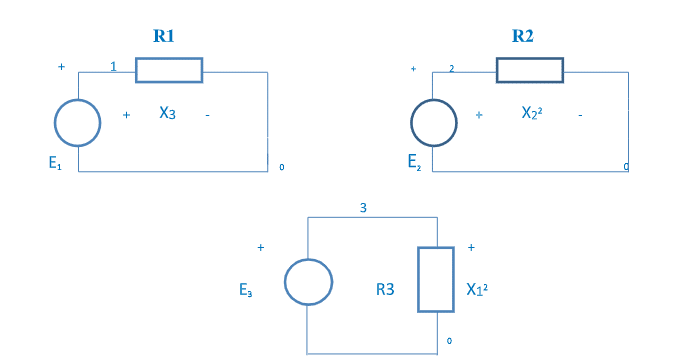
The following describe Pspice circuit file TABLE I to solve the already mentioned non-linear equations (set 1) in three variables,
TABLE I
| **** 08/23/22 13:13:50 ****** PSpice Lite (October 2012) ****** ID# 10813 **** |
| To verify using analogue behaviour modelling Pspice |
| **** Circuit description |
| ****************************************************************************** |
| R1 1 0 1 |
| R2 2 0 1 |
| R3 3 0 1 |
| E1 1 0 VALUE={-((SQRT(V(3))+SQRT(V(2)))**2-SQRT(V(3))*SQRT(V(2))-10)} |
| E2 0 3 VALUE={SQRT(V(3))*V(1)-4.} |
| E3 2 0 VALUE={12-2.*(SQRT(V(3))+V(1))} |
| E4 4 0 VALUE={SQRT(V(3))} |
| R4 4 0 1 |
| E5 5 0 VALUE={SQRT(V(2))} |
| R5 5 0 1 |
| * VALUE OF X1 IS VOLTAGE ACROSS R4 |
| *VALUE OF X2 IS VOLTAGE ACROSS R5 |
| *VALUE OF X3 IS VOLTAGE ACROSS R1 |
| .END |
| **** 08/23/22 13:13:50 ****** PSpice Lite (October 2012) ****** ID# 10813 **** |
| To verify using analogue behaviour modelling Pspice |
| **** Small signal bias solution Temperature = 27.000 DEG C |
| ****************************************************************************** |
| Node voltage Node voltage Node voltage Node voltage |
| ( 1) 3.0000 ( 2) 4.0000 ( 3) 1.0000 ( 4) 1.0000 |
| ( 5) 2.0000 |
Case 1:
Consider equation (1) with
K1=K2=K3=K4=K5=K8=K7=1
(x1+x2) 2 – x1.x2+ x3=10
x1.x3 + ( x1)2 =4 ….(1)
(x2)2 + 2.(x1+x3) = 12
The PSpice file to solve this set with analogue behavioural voltage sources is given in Table I.
Case 2:
Consider equation (1) with
K1=K2=1, K3=-1,K4=1,K5=-1=K6 K7=1
(x1+x2) 2 – x1.x2- x3=10
x1.x3 -( x1)2 =4 ….(2)
-(x2)2 + 2.(x1+x3) = 12
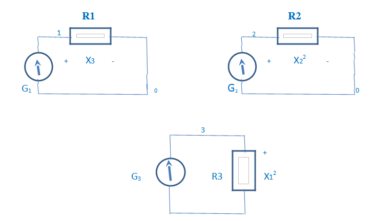
TABLE II
| *** 07/07/23 16:19:39 ****** PSpice Lite (October 2012) ****** ID# 10813 **** |
| Solution to non-linear equations by current concept |
| **** Circuit description |
| ****************************************************************************** |
| R1 1 0 1 |
| R2 2 0 1 |
| R3 3 0 1 |
| GE1 6 0 VALUE={-((SQRT(I(V38))+SQRT(I(V27)))**2-SQRT(I(V38))*SQRT(I(V27))-10)} |
| V16 6 1 |
| GE2 0 8 VALUE={SQRT(I(V38))*I(V16)-4.} |
| V38 8 3 |
| GE3 7 0 VALUE={12-2.*(SQRT(I(V38))+I(V16))} |
| V27 7 2 |
| GE4 0 4 VALUE={SQRT(I(V38))} |
| R4 4 0 1 |
| GE5 0 5 VALUE={SQRT(I(V27))} |
| R5 5 0 1 |
| * VALUE OF X1 IS VOLTAGE ACROSS R4 |
| *VALUE OF X2 IS VOLTAGE ACROSS R5 |
| *VALUE OF X3 IS VOLTAGE ACROSS R1 |
| **** 07/07/23 16:19:39 ****** PSpice Lite (October 2012) ****** ID# 10813 **** |
| Solution to non-linear equations by current concept |
| **** Small signal bias solution Temperature = 27.000 DEG C |
| ****************************************************************************** |
| Node voltage Node voltage Node voltage Node voltage |
| ( 1) 1.5244 ( 2) -6.1950 ( 3) -1.8992 ( 4) 1.3781 |
| ( 5) 2.4890 ( 6) 1.5244 ( 7) -6.1950 ( 8) -1.8992 |
| Voltage source currents |
| NAME CURRENT |
| V16 1.524E+00 |
| V38 -1.899E+00 |
| V27 -6.195E+00 |
| Total power dissipation 0.00E+00 WATTS |
| Job concluded |
The Pspice file to solve this set with analogue behavioural current sources is given in TABLE II with solutions.
Case 3:
The Pspice file to solve the set(1) with analogue behavioural current sources is given in TABLE III
TABLE III
| **** 07/07/23 16:26:01 ****** PSpice Lite (October 2012) ****** ID# 10813 **** |
| Solution to non-linear equations by current concept |
| **** Circuit description |
| ****************************************************************************** |
| R1 1 0 1 |
| R2 2 0 1 |
| R3 3 0 1 |
| GE1 0 6 VALUE={-((SQRT(I(V38))+SQRT(I(V27)))**2-SQRT(I(V38))*SQRT(I(V27))-10)} |
| V16 6 1 |
| GE2 8 0 VALUE={SQRT(I(V38))*I(V16)-4.} |
| V38 8 3 |
| GE3 0 7 VALUE={12-2.*(SQRT(I(V38))+I(V16))} |
| V27 7 2 |
| GE4 0 4 VALUE={SQRT(I(V38))} |
| R4 4 0 1 |
| GE5 0 5 VALUE={SQRT(I(V27))} |
| R5 5 0 1 |
| * VALUE OF X1 IS VOLTAGE ACROSS R4 |
| *VALUE OF X2 IS VOLTAGE ACROSS R5 |
| *VALUE OF X3 IS VOLTAGE ACROSS R1 |
| .END |
| **** 07/07/23 16:26:01 ****** PSpice Lite (October 2012) ****** ID# 10813 **** |
| Solution to non-linear equations by current concept |
| **** Small signal bias solution Temperature = 27.000 DEG C |
| ****************************************************************************** |
| Node voltage Node voltage Node voltage Node voltage |
| ( 1) 3.0000 ( 2) 4.0000 ( 3) 1.0000 ( 4) 1.0000 |
| ( 5) 2.0000 ( 6) 3.0000 ( 7) 4.0000 ( 8) 1.0000 |
| Voltage source currents |
| Name Current |
| V16 3.000E+00 |
| V38 1.000E+00 |
| V27 4.000E+00 |
Case 4:
Consider the set of equations (1) with K1=K2=K3=K4=1,K5=-1
| TABLE IV Solution to non-linear equations by current concept |
| **** Circuit description |
| ****************************************************************************** |
| R1 1 0 1 |
| R2 2 0 1 |
| R3 3 0 1 |
| GE1 0 6 VALUE={-((SQRT(I(V38))+SQRT(I(V27)))**2-SQRT(I(V38))*SQRT(I(V27))-10)} |
| V16 6 1 |
| GE2 8 0 VALUE={SQRT(I(V38))*I(V16)-4.} |
| V38 3 8 |
| GE3 0 7 VALUE={12-2.*(SQRT(I(V38))+I(V16))} |
| V27 7 2 |
| GE4 0 4 VALUE={SQRT(I(V38))} |
| R4 4 0 1 |
| GE5 0 5 VALUE={SQRT(I(V27))} |
| R5 5 0 1 |
| * VALUE OF X1 IS VOLTAGE ACROSS R4 |
| *VALUE OF X2 IS VOLTAGE ACROSS R5 |
| *VALUE OF X3 IS VOLTAGE ACROSS R1 |
| .END |
| **** 07/07/23 16:28:22 ****** PSpice Lite (October 2012) ****** ID# 10813 **** |
| Solution to non-linear equations by current concept |
| **** Small signal bias solution Temperature = 27.000 DEG C |
| ****************************************************************************** |
| Node voltage Node voltage Node voltage Node voltage |
| ( 1) 6.3489 ( 2) -2.1163 ( 3) -.5031 ( 4) .7093 |
| ( 5) 1.4547 ( 6) 6.3489 ( 7) -2.1163 ( 8) -.5031 |
| Voltage source currents |
| Name Current |
| V16 6.349E+00 |
| V38 5.031E-01 |
| V27 -2.116E+00 |
| Total power dissipation -0.00E+00 WATTS |
| Job concluded |
Case 5:
Consider the set of equations (1) with
K1=K2=K3=K4=1, K5=-1
K6=K7=1
(x1+x2) 2 – x1.x2+ x3=10
(x2)2 + 2.(x1+x3) = 12
The Pspice file to solve this set with analogue behavioural current sources is given in TABLE V with solved answers
TABLE V
| **** 07/07/23 16:31:37 ****** PSpice Lite (October 2012) ****** ID# 10813 **** |
| Solution to non-linear equations by current concept |
| **** Circuit description |
| ****************************************************************************** |
| R1 1 0 1 |
| R2 2 0 1 |
| R3 3 0 1 |
| GE1 0 6 VALUE={-((SQRT(I(V38))+SQRT(I(V27)))**2-SQRT(I(V38))*SQRT(I(V27))-10)} |
| V16 6 1 |
| GE2 8 0 VALUE={SQRT(I(V38))*I(V16)-4.} |
| V38 8 3 |
| GE3 0 7 VALUE={12-2.*(SQRT(I(V38))+I(V16))} |
| V27 7 2 |
| GE4 0 4 VALUE={SQRT(I(V38))} |
| R4 4 0 1 |
| GE5 0 5 VALUE={SQRT(I(V27))} |
| R5 5 0 1 |
| * VALUE OF X1 IS VOLTAGE ACROSS R4 |
| *VALUE OF X2 IS VOLTAGE ACROSS R5 |
| *VALUE OF X3 IS VOLTAGE ACROSS R1 |
| .END |
| **** 07/07/23 16:31:37 ****** PSpice Lite (October 2012) ****** ID# 10813 **** |
| Solution to non-linear equations by current concept |
| **** Small signal bias solution Temperature = 27.000 DEG C |
| ****************************************************************************** |
| Node voltage Node voltage Node voltage Node voltage |
| ( 1) 3.0000 ( 2) 4.0000 ( 3) 1.0000 ( 4) 1.0000 |
| ( 5) 2.0000 ( 6) 3.0000 ( 7) 4.0000 ( 8) 1.0000 |
| Voltage source currents |
| Name Current |
| V16 3.000E+00 |
| V38 1.000E+00 |
| V27 4.000E+00 |
| Total power dissipation -0.00E+00 WATTS |
| Job concluded |
(b) Non-Linear two variable trigonometry simultaneous equations
Consider the following non-linear trigonometric two variable functions
C1.X12 – 2.C2.* sin(X2)+C3.X1*X2= 5.14158
C4.X2 – C5.X1*X2 = -1.570796
The following TABLE VI describes PSPICE circuit file and results for this set of non-linear equations in two variables,
TABLE VI
| **** 08/24/22 18:58:09 ****** PSpice Lite (October 2012) ****** ID# 10813 **** |
| To verify using analogue behaviour modelling Pspice |
| **** CIRCUIT DESCRIPTION |
| ****************************************************************************** |
| *C1=C2=C3=C4=C5=1 R1 1 0 1 |
| R2 2 0 1 |
| E1 1 0 VALUE={2.*sin(V(2))-SQRT(V(1))*V(2)+5.14159} |
| E2 2 0 VALUE={-1.570796+SQRT(V(1))*V(2)} |
| E3 3 0 VALUE={SQRT(V(1))} |
| R3 3 0 1 |
| E5 5 0 VALUE={SIN(1.570796)} |
| R5 5 0 1 |
| EVERIFY 7 0 VALUE={1.6999**2-2*sin(2.24444)+1.6999*2.2444} |
| R70 7 0 1 |
| EVERIFY2 8 0 VALUE={2.2444-1.6999*2.2444} |
| R8 8 0 1 |
| EVERY 9 0 VALUE={2**2-2.*SIN(1.570796)+2.*1.570796} |
| R9 9 0 1 |
| EVERQ 10 0 VALUE={1.570796-2.*1.570796} |
| R10 10 0 1 |
| *VALUE OF X1 IS VOLTAGE ACROSS R3 |
| *VALUE OF X2 IS VOLTAGE ACROSS R2 |
| .END |
| **** 08/24/22 18:58:09 ****** PSpice Lite (October 2012) ****** ID# 10813 **** |
| To verify using analogue behaviour modelling Pspice |
| **** Small signal bias solution Temperature = 27.000 DEG C |
| ****************************************************************************** |
| Node voltage Node voltage Node voltage Node voltage |
| ( 1) 2.8896 ( 2) 2.2444 ( 3) 1.6999 ( 5) 1.0000 |
| ( 7) 5.1418 ( 8) -1.5709 ( 9) 5.1416 ( 10) -1.5708 |
Now consider a different set of two variable non-linear trigonometric equations in X, Y,
X = 2.*sin(Y) – A1* sqrt(abs(X)) . Y + 5.14159
Y= -1.570796 + A2*sqrt(abs(X)) . Y
The following TABLE VII describes to solve these equations and the results are also given in the form of voltages.
TABLE VII
| **** 08/26/22 09:13:32 ****** PSpice Lite (October 2012) ****** ID# 10813 **** |
| To verify using analogue behaviour modelling Pspice |
| **** Circuit Description |
| ****************************************************************************** |
| *A1=A2=1 R1 1 0 1 |
| R2 2 0 1 |
| E1 1 0 VALUE={2.*sin(V(2))-SQRT(V(1))*V(2)+5.14159} |
| E2 2 0 VALUE={-1.570796+SQRT(V(1))*V(2)} |
| E3 3 0 VALUE={SQRT(V(1))} |
| R3 3 0 1 |
| *VALUE OF X1 IS VOLTAGE ACROSS R1 |
| *VALUE OF X2 IS VOLTAGE ACROSS R2 |
| .END |
| **** 08/26/22 09:13:32 ****** PSpice Lite (October 2012) ****** ID# 10813 **** |
| To verify using analogue behaviour modelling Pspice |
| **** Small signal bias solution Temperature = 27.000 DEG C |
| ****************************************************************************** |
| Node voltage Node voltage Node voltage Node voltage |
| ( 1) 2.8896 ( 2) 2.2444 ( 3) 1.6999 |
Consider a different set of non-linear equations in two variables as described below,
-X12 = 2.B1. SIN(X2) – sqrt(abs(X12)) .X2 + 5.14159
-X2 = -1.570796 +B2. sqrt(abs(X12)) .X2
TABLE VII describes the PSpice circuit schematic to solve these equations with results.
TABLE VII
| **** 08/26/22 09:37:32 ****** PSpice Lite (October 2012) ****** ID# 10813 **** |
| To verify using analogue behaviour modelling Pspice |
| **** Circuit Description |
| ****************************************************************************** |
| *B1=B2=1 R1 1 0 1 |
| R2 2 0 1 |
| E1 4 0 VALUE={ABS(V(1))} |
| R40 4 0 1 |
| G1 1 0 VALUE={2.*sin(V(2))-SQRT(V(4))*V(2)+5.14159} |
| G2 2 0 VALUE={-1.570796+SQRT(V(4))*V(2)} |
| G3 3 0 VALUE={SQRT(V(1))} |
| R3 3 0 1 |
| *Result verification |
| G4 5 0 VALUE={2*sin(.4857)-SQRT(4.9902)*.4857+5.14159} |
| R50 5 0 1 |
| G5 6 0 VALUE={-1.570796+SQRT(4.9902)*.4857} |
| R60 6 0 1 |
| *VALUE OF X1 IS VOLTAGE ACROSS R3 |
| *VALUE OF X2 IS VOLTAGE ACROSS R2 |
| .END |
| **** 08/26/22 09:37:32 ****** PSpice Lite (October 2012) ****** ID# 10813 **** |
| To verify using analogue behaviour modelling Pspice |
| **** Small signal bias solution Temperature = 27.000 DEG C |
| ****************************************************************************** |
| Node voltage Node voltage Node voltage Node voltage |
| ( 1) -4.9902 ( 2) .4857 ( 3) -2.2339 ( 4) 4.9902 |
| ( 5) -4.9903 ( 6) .4858 |
In conclusion, the effective use of PSpice’s analogue behaviour modelling option is invaluable for solving sets of non-linear multi-variable equations using circuit theory principles and applying dependent current and voltage sources.
Reference
- K. Bharath kumar, Cascaded Transmission Parameters from PSPICE Circuit Simulation, issue
8, Vol. 5, All About Electronics Magazine, pp. 51-58, June 2023, published. - PSpice Manual. Irvine, California: MicroSim Corporation, 1992.
- K. Bharath Kumar, “Techniques for Using SPICE to derive Thevenin and Norton equivalent
circuits”, EDN (edn.com), Design Ideas, February 14, 2022. - K. Bharath Kumar, “Using Substitution Theorem to derive Thevenin resistance values with
SPICE”, EDN(edn.com), Design Ideas, September 10, 2021. - Paul Tuinenga, SPICE: A Guide to Circuit Simulation and Analysis Using PSpice,3d. Englewood
Cliffs, New Jersey:Prentice Hall, 1995. - Andrei Vladimirescu,The Spice Book. New York:John Wiley & Sons, 1994.
The author obtained a B. Tech degree in E & CE with the highest honours from JNT University, Anantapur, India, in 1981. He later earned an M.Tech degree from the Indian Institute of Technology, Kharagpur, India, in the area of Microwave and Optical Communication in 1983. Subsequently, he joined the Indian Telephone Industries in Bangalore, India, where he worked in the field of fibre optics. In 1990, he obtained an M.S. degree in electrical engineering from the Illinois Institute of Technology, Chicago, USA, and joined Oki Electric in Japan as a researcher in the semiconductor laboratory. He has authored over twenty publications in the area of simulation and modelling of electronic circuits in various national and international journals. He is now retired from Oki Electric, Japan.