 The basic setup needed to receive the weather satellites was covered in ‘Set Up Your Own Weather Satellite Receiving Station’ article published in January issue. The antenna setup, the receivers, and decoding software were discussed in detail in that article. By this time, the author hopes that many readers would have their receiving stations up and running.
In this article, we shall look at the imaging systems of these satellites and how the automatic picture transmission (APT) protocol works. Later we shall see how to decode the digital QPSK transmission from the Russian Meteor M2 satellite and produce even higher resolution earth imagery.

 It should be noted that the APT transmission is being phased out and the currently operational satellites, such as NOAA-15, NOAA-18, and NOAA-19, are the last ones to carry such analogue transmission payload. But why discuss this phased out system when digital transmission, such as Meteor, is readily available?
Many universities and academic institutions all over the world are building nano satellites (Cube Sats). Therefore, one can think of how meaningful and scientific imaging data can still be transmitted using such narrow-band protocol. May be some groups active with the nano satellites can work towards such an experiment in the future Cube Sat missions!
The present scope of discussion is:
- Basic imaging process onboard NOAA satellites
- The high-resolution picture transmission (HRPT) and low-resolution analogue APT transmission protocol
- Receiving and decoding weather images from Russian Meteor M2 satellite
Basic imaging process
The images that we receive from these earth imaging satellites are generally a result of what is called scanning radio meter, an instrument that produces the output to the corresponding intensity of the spectral components through scanning. It utilises a mirror that rotates at angular speed of 360rpm and reflects the energy received from various lenses to the spectral sensors.
As the satellite progresses through its orbital path, the reflected energy received perpendicular to the satellite’s trajectory is used to construct each line of the image. Thus, a complete two-dimensional image of the area over which the satellite passes is constructed.
As the mirror rotates during each scan, the sensors look at the earth using the mirror and lens arrangement. These sensors are calibrated on-the-fly during each line with respect to emission from the Deep Sky and Black-Body radiation on board the spacecraft as a reference. This entire instrumentation is called very high resolution radio meter (VHRR).
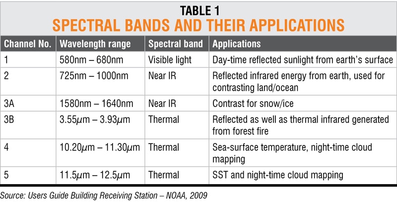
Table 1 summarises the various spectral bands and their primary applications.
As the energy/emission falls on these sensors, electrical signal is produced, which is further digitised by an analogue-to-digital converter (ADC) with a resolution of 10 bits, thereby producing an equivalent of 1024 grey-scale levels.
The transmission protocols
HRPT transmission
With a high-resolution picture transmission (HRPT) protocol, this image data is transmitted at 360 lines per minute and each of the scan line produces 2048 pixels per line. Since this is a very huge data, the signal is transmitted digitally at a 665kbps rate with PSK modulation at main carrier frequencies of 1698MHz, 1708MHz, or 1702.5MHz. Therefore, the ground-receiving station becomes complex for an individual or amateur experimenter to construct. Each line has a pixel resolution of 1.1km and the HRPT image is transmitted using all the above five channels.
APT analogue transmission
The automatic picture transmission (APT) protocol is the one we are currently using to receive images from the NOAA satellites. However, only two channels from the above five sensors are used for APT transmission, which are decided by the ground command-and-control of the satellite and thus are not user-selectable.
From the 10-bit ADC, the APT uses 8-bit MSB data to produce the 8-bit grey-scale levels for the analogue APT transmission. It uses a 2.4kHz audio tone and its amplitude is modulated as a function of the intensity level (grey-scale level) of the picture information. Also, the HRPT produces 360 lines per minute from which only two lines from the spectral channels are used for producing the APT data. Therefore, the resulting line resolution gets reduced to 120 lines per minute.
Thus, with 120 lines per minute, we get two lines per second, or each line has a 0.5-second (500ms) duration. Let us now see how these 500ms get distributed between various signal components, as shown in Fig. 1.
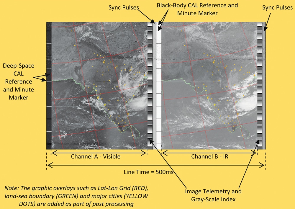
- The sync pulses. The sync pulses are transmitted in the form of square wave pulses for each set of the image component, that is, the Visible channel and the IR channel. Each set consists of seven pulses. For the Visible image channel, 1040Hz square wave pulses are used. While for the IR channel, 832Hz square wave pulses are used. These sync pulses appear as vertical lines in the primary raw image data received from the satellite and can be seen in Fig. 1 at the middle and right hand side of the image.
- CAL references and time markers. The scanner uses two references while scanning the earth. It uses the Deep Space as a reference for the channel A visible imagery, and it appears as a vertical black strip at the beginning of the Visible channel, as can be seen at the left hand side of the image. Also, horizontal white lines are overlaid for time reference as 1-Minute Marker.For the channel B IR imagery, the Black-Body is used as the thermal reference and appears as vertical white strip at the beginning of the IR channel. Similarly, the time markers are overlaid as 1-Minute Marker but appear as black horizontal lines, as can be seen in the mid-right part of Fig. 1.
- Telemetry data and grey-scale indices. For each of the Visible and IR channel, the image brightness data is transmitted as varying grey-scale levels and appear as horizontal strips called Wedges. It is used for temperature calibration of the image data in the respective image channel.
- Channel A (Visible sensor) image. The channel A image section appears for 250ms of the scan-line from the Visible sensor of the satellite. Besides the CAL reference and the telemetry data, the major part contains the image data. During the earth scan, the visible light reflected from the earth’s surface is used to construct this image. It therefore contains the oceans appearing as black, the clouds appearing as white, and the land as various levels of grey scale.During night-time, this channel sends image data from another IR channel and has a clear and distinct image difference as compared to channel B’s IR image data. The ground control decides the channel to be used during night-time pass of the satellite.
- Channel B (IR sensor) image. Similarly, the channel B image section appears for the remaining of the 250ms and sends data from the IR sensor. Apart from the sync and telemetry data, the remainder of the time is used to send the sensor data from earth scan. Warmer objects appear as black or darker grey shades while colder objects appear white or lighter shades.
With the present scope of the article and space limitation, it is not possible to entirely cover the APT image format, but when receiving these images, it is equally important to understand the image data properly. Therefore, this section has been limited to the basic information only. Readers are advised to refer to the NOAA website for further information.
Receiving and decoding weather images
The APT offers us a resolution of 4km/pixel. Also, there is the Meteor M2 satellite from Russia that transmits the earth imagery in the same 137MHz weather band, currently at 137.1MHz but in digital format at 72kbps QPSK. It offers even higher resolution of 1km/pixel in stunning three spectral bands as against only two channels from the NOAA APT.
Therefore, the decoding software WXtoImg used in the first article is unsuitable for this satellite. We require both the QPSK demodulator and the image extractor from the demodulated data.
The imager in Meteor is called MSU-MR or MultiSpectral Scanner for meteorological purposes. Table 2 summarises the spectral bands comparison of NOAA and Meteor M2 satellites.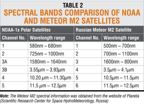
Software options
Since this satellite offers higher resolution of 1km/pixel, let us now see how to demodulate the signal and obtain the earth imagery.
There are two options, and both require manual processing or file handling. Nothing gets automatically processed like the analogue APT software that we use for NOAA satellites. The options are:
Option 1: SDR# software with built-in Meteor M2 demodulator
Option 2: Manually recording the SDR I/Q data in a file and then processing it
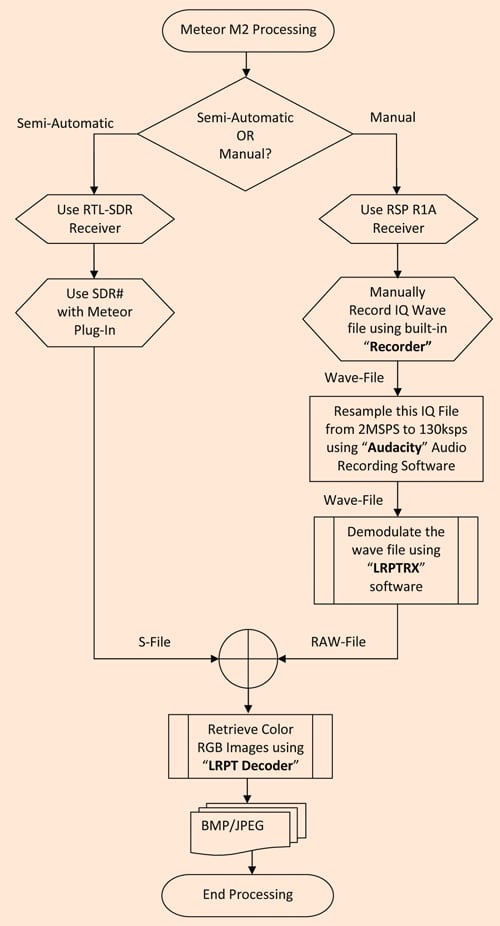
Both these options give a demodulated output file, which needs to be processed manually to get the RGB colour/spectral images from the demodulated data. Fig. 2 illustrates a flow-chart for both these options.
The RTL-SDR with SDR# software and Meteor plug-in
The readers should familiarise themselves with the installation and usage of the SDR# software from AirSpy for use with the RTL-SDR receiver and, more importantly, the Meteor plug-in. One can download the SDR# software and add the plug-in later or download the latest version of the software from www.airspy.com.
The author is grateful to Alex of the HappySatl.nl website and Les Hamilton of the UK. Their articles are very useful for setting up the Meteor satellite demodulation and processing software properly.
Given below are the steps to set up the software to receive the satellite signals:
Step 1: Receiver preparation and settings. The Meteor demodulator is a QPSK soft demodulator. Also, the software defined radio is nothing but an ADC sampling the RF signal at some high rates of >1MSPS (mega samples per second).
Therefore, we need some settings at the SDR sampling rate as well for the demodulator to work properly. After studying various published information, we had set the RTL-SDR sampling rate at 1.4MSPS, somewhere in between 1MSPS and 2MSPS. This can be achieved by clicking the Configure Source button on the SDR# main menu at the top. A dialogue box appears, as shown in Fig. 3(a). Maintain settings accordingly with the RTL AGC box unticked and Tuner AGC RF Gain set to the maximum. The oscillator frequency correction needs to be set around 70ppm, or the value specified by the manufacturer, for better frequency stability.
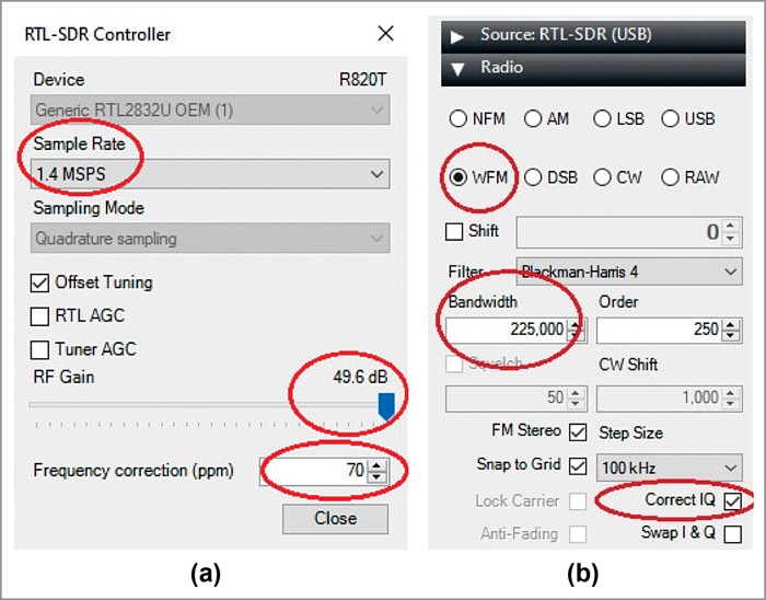
Next, set the radio receiver in wide-band FM (WFM) with a bandwidth of around 225kHz and tick the Correct I/Q check box, as shown in Fig. 3(b).
Step 2: The Meteor demodulator settings. Setup the demodulator plug-in. If your demodulator plug-in is successfully installed, it appears in your list as shown in Fig. 4(a). When you click on it, you should see the demodulator settings, as shown in Fig. 4(b).
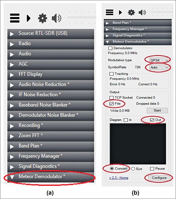
As shown in Fig. 4(b), set the modulation as QPSK and the symbol rate to either 72k or auto. Uncheck the Demodulator and Tracking boxes at this stage. The tracking option is utilised when the Doppler shifts in frequency or in conjunction with an automatic antenna tracker. The demodulator check-box enables or disables the demodulator and can be used at the time of receiving the satellite.
For output settings, check the File check-box, so that the demodulator writes the demodulated data as a file. The folder or location where this file will be stored is set using the Configure settings at the bottom-right of the diagram. When the demodulator starts writing data to the file, it will show the data size being written to the file. For a successful satellite file this data can range from 36MB to all the way up to 70MB large data files!
The demodulator is an excellent diagnostic tool, which can be found very useful when a satellite signal is being received. In the Diagram option, we can choose the input side or output side signal quality as the Constellation or Eye diagrams. The Constellation diagram is an easy diagnostic tool, as can be seen later when actual signal is received, as it shows the four phases (Quadrature Phase Modulation!) and magnitudes in each of the four quadrants.
Step 3: Recording a satellite pass. The final step in the first approach is to record the actual satellite pass. For this, we know the Meteor M2 satellite transmits at 137.100MHz. Find the satellite pass from your Prediction software, tune the receiver to this frequency, and start the demodulator by checking the Demodulator check-box, as shown in Fig. 5(a). As the satellite rises above horizon, the signal strength increases, and you shall see that the Constellation diagram starts changing from random dots to a circular ‘O’ ring and then finally stabilises with four dots indicating that the 72kHz QPSK signal is being received.
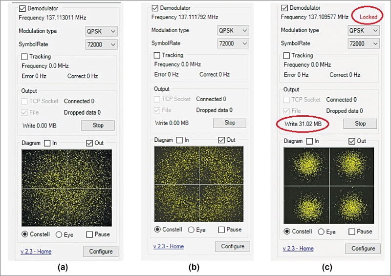
At the same time two important developments take place. First, the demodulator shows a ‘Locked’ status in red colour and the File Write shows the data being written to the file. Refer Fig. 5(b) and Fig. 5(c). When the satellite leaves your horizon or field of view, the demodulator also loses lock onto the carrier and any data write also ceases. For a good and successful satellite pass, one can expect a file size in excess of 60MB, although smaller file sizes of 35MB are also possible and would result in useful earth imagery.
Once your satellite pass is complete, stop the demodulator and uncheck the Demodulator check-box. The demodulated data file is saved with a ‘.S’ extension in the folder you chose while configuring the demodulator.
Since the image extraction process is common to both approaches, we shall see this process at a later point in the text.
Manual recording using IQ wave file
The other method is to manually record the IQ signal in the form of a .wave file and then demodulate it as part of the post processing. Although this is a very cumbersome and time consuming process, sometimes it proves advantageous.
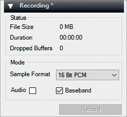
Step 1: Recording the satellite pass using the I-Q wave file. Whether you are using the RTL-SDR with the SDR# or the RSP1A receiver with SDRUno software, both these receiver GUIs offer you a facility to record the sound or the baseband I-Q (Quadrature Modulation) data as a wave file. Refer Fig. 6 for this. Kindly note that this wave file is the actual RF signal recorded and not a demodulated output.

Step 2: Processing the wave file using Audacity. The next step is to resample the recorded RF signal at a lower sampling rate. This is necessary for the demodulation process in the next step. For this, open the satellite wave file (I-Q data) in Audacity software.
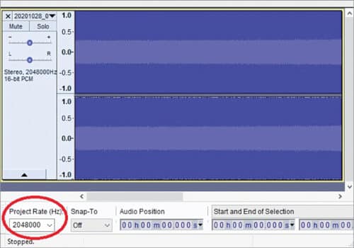
The file might be large, several GB in size! And you can notice the sampling rate at which the SDR recorded this wave file in the bottom left corner of the Audacity GUI. Refer Fig. 7 for details.
Next, change this sampling to 130ksps. For example, if your sampling rate is shown as 2048000, change it to 130000. Then, select the entire waveform/signal and save the File/data as (Save as…) wave file. Once saved properly, you would notice that the file size has reduced from GBs to a few hundred MBs. You can delete the larger files to save space on the hard disk as these are not needed any more.
Step 3: Manually demodulating the wave file. The next step is to demodulate this wave file using the LrptRx Demodulator software, which the author found from the websites mentioned above. The link is: https://www.dropbox.com/s/qq1fjyitpa3j14o/software.zip
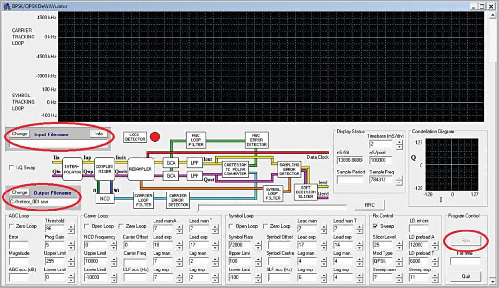
The dashboard of LRPTRX, as shown in Fig. 8(a), is very complex but we do not have to worry about that. We just need to enter the Input and Output filenames and their locations. Then hit the Run button highlighted in Fig. 8(a). Kindly note that the output file is a .RAW, while the Meteor demodulator plug-in produces a .S file as the output file. However, as shown in the flow-chart in Fig. 2, both these files are acceptable for this project.
It should be noted that this is a long process, which takes almost double the time the satellite pass takes. While the demodulator processes the data files, it shows the carrier demodulation process and, if the satellite has been received properly, the Lock Detector (red dot in Fig. 8(a)) turns green and also the Constellation Diagram towards the right starts showing the four phase-amplitude dots of the QPSK signal, as illustrated in Fig. 8(b).
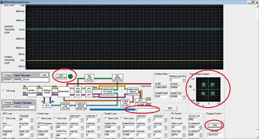
As the demodulation progresses, the status/progress bar also slides towards right. The only problem with this software is that it does not stop automatically, even after all the file data has been processed. You need to press the Stop button to stop it and then quit the program.
This completes the manual demodulation processes. Next, we shall see the final step that is applicable to both the approaches, that is, to extract the actual image file(s) from this demodulated data.
Image extraction, the final step
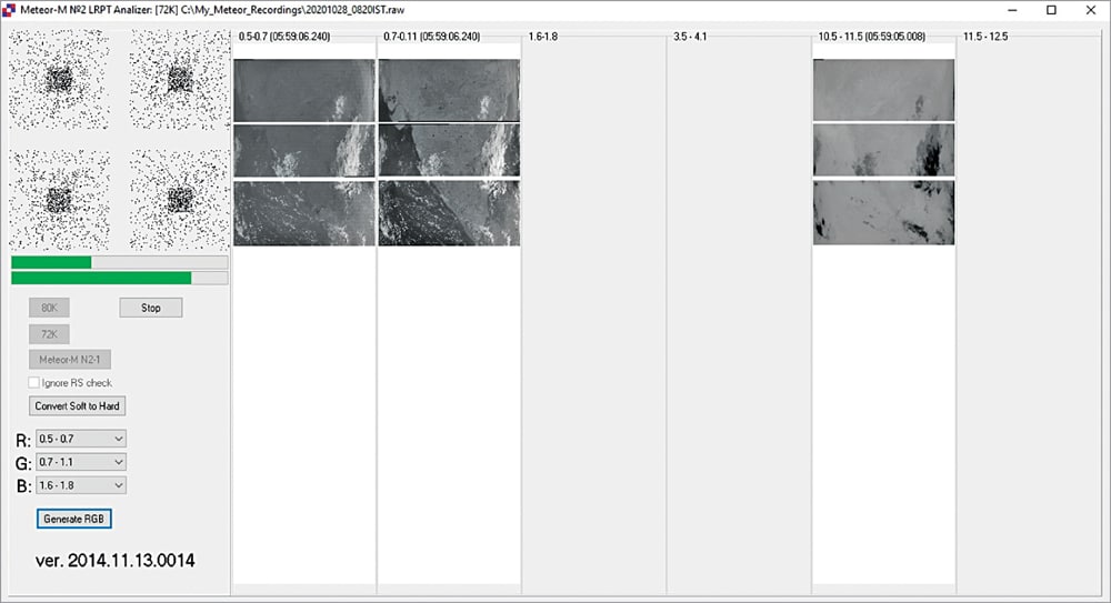
This is the final step in our effort to demodulate the earth imagery from the Meteor satellite data. From the above discussions, either through the plug-in or through the manual demodulation, we get the .S or the .RAW file. At this stage, we shall require the Off-line Meteor LRPT Analyser software, as mentioned earlier in this article.
Click on the 72k button in LRPT Analyser/Decoder software and the file selection dialogue box opens. Choose either S file or RAW file. The software starts and shows the constellation diagram. If it finds the data properly, you shall see the grey-scale images displayed from the three active bands as sent by the Meteor satellite. Out of these three, there will be two in the visible/near-IR region. The third channel is switched depending upon the season to monitor the snow in the higher latitude countries during winter-time.
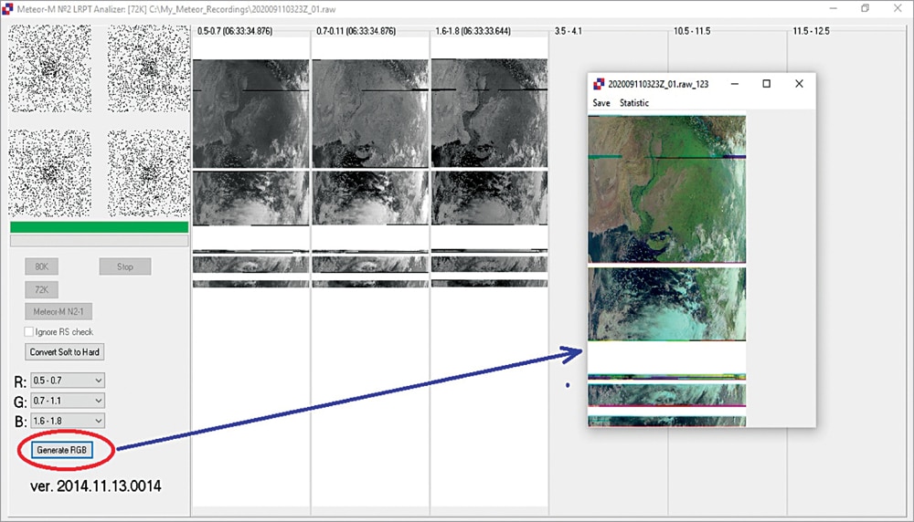
Once the decryption process is completed, you can click on the Generate RGB button and the image will be produced. Refer Fig. 9(a) and Fig. 9(b).
Conclusion
Images from each of these satellites, the NOAA satellites with Analogue APT weather imagery and the high resolution images from the Meteor M2, are quite useful for understanding the weather, cloud patterns, and cyclones. The author has also been experimenting with various antennas, impedance matching, and the antenna pre-amplifier for making this reception better in the best possible way and within acceptable budgets! For a successful reception, a proper antenna and good cabling system is equally important.
Prasanna Waichal holds a master’s degree in electronics and has more than 25 years of work experience in industrial R&D for design and development of specialised and strategic electronics systems and academic teaching and research at post-graduate levels, both in India and abroad. His passions include radio reception and studying solar activities and their effect on ionosphere on earth. He is also a licensed amateur radio operator with call-sign VU3OOI. He claims to have discovered a method to predict earthquakes using very-low-frequency (VLF) multipath-multi-frequency propagation technique