


Image processing covers a wide and diverse array of techniques and algorithms. Fundamental processes underlying these techniques include sharpening, noise removal, deblurring, edge extraction, binarisation, contrast enhancement, and object segmentation and labeling.
Sharpening enhances the edges and fine details of an image for viewing by human beings. It increases the contrast between bright and dark regions to bring out image features. Basically, sharpening involves application of a high-pass filter to an image.

Noise removal techniques reduce the amount of noise in an image before it is processed any further. It is necessary in image processing and image interpretation so as to acquire useful information. Images from both digital cameras as well as conventional film cameras pick up noise from a variety of sources. These noise sources include salt-and-pepper noise (sparse light and dark disturbances) and Gaussian noise (each pixel value in the image changes by a small amount). In either case, the noise at different pixels can either be correlated or uncorrelated. In many cases, noise values at different pixels are modeled as being independent and identically distributed and hence uncorrelated. In selecting noise reduction algorithm, one must consider the available computer power and time and whether sacrificing some image detail is acceptable if it allows more noise to be removed and so on.
Deblurring is the process of removing blurring artifacts (such as blur caused by defocus aberration or motion blur) from images. The blur is typically modelled as a convolution point-spread function with a hypothetical sharp input image, where both the sharp input image (which is to be recovered) and the point-spread function are unknown. Deblurring algorithms include methodology to remove the blur from an image. Deblurring is an iterative process and you might need to repeat the process multiple times until the final image is the best approximation of the original image.
Edge extraction or edge detection is used to separate objects from one another before identifying their contents. It includes a variety of mathematical methods that aim at identifying points in a digital image at which the image brightness changes sharply.
Edge detection approaches can be categorised into search-based approach and zero-crossing-based approach. Search based methods detect edges by first computing a measure of edge strength (usually a first-order derivative function) such as gradient magnitude and then searching for a local directional maxima of the gradient magnitude using a computed estimate of the local orientation of the edge, usually the gradient direction. Zero-crossing methods look for zero-crossings in a second-order derivative function computed from the image to find the edge. First-order edge detectors include Canny edge detector, Prewitt and Sobel operators, and so on.
Other approaches include second-order differential approach of detecting zero-crossings, phase congruency (or phase coherence) methods or phase-stretch transform (PST). Second-order differential approach detects zero-crossings of the second-order directional derivative in the gradient direction. Phase congruency methods attempt to find locations in an image where all sinusoids in the frequency domain are in phase. PST transforms the image by emulating propagation through a diffractive medium with engineered 3D dispersive property (refractive index).
Binarisation refers to reducing a greyscale image to only two levels of grey, i.e., black and white. Thresholding is a popular technique for converting any greyscale image into a binary image.
Contrast enhancement is done to improve an image for human viewing as well as for image processing tasks. It makes the image features stand out more clearly by making optimal use of colours available on the display or the output device. Contrast manipulation involves changing the range of contrast values in an image.
Segmentation and labeling of objects within a scene is a prerequisite for most object recognition and classification systems. Segmentation is the process of assigning each pixel in the source image to two or more classes. Image segmentation is the process of partitioning the digital image into multiple segments (sets of pixels, also known as super pixels). The goal is to simplify and/or change the contrast representation of an image into something that is more meaningful and easier to analyse. Once the relevant objects have been segmented and labelled, their relevant features can be extracted and used to classify, compare, cluster or recognise desired objects.
Types of images
The MATLAB tool box supports four types of images, namely, grey-level images, binary images, indexed images and RGB images. Brief description of these image types is given below.
Grey-level images
Also referred to as monochrome images, these use 8 bits per pixel, where a pixel value of 0 corresponds to ‘black,’ a pixel value of 255 corresponds to ‘white’ and intermediate values indicate varying shades of grey. These are also encoded as a 2D array of pixels, with each pixel having 8 bits.
Binary images
These images use 1 bit per pixel, where a 0 usually means ‘black’ and a 1 means ‘white.’ These are represented as a 2D array. Small size is the main advantage of binary images.
Indexed images
These images are a matrix of integers (X), where each integer refers to a particular row of RGB values in a secondary matrix (map) known as a colour map.
RGB image
In an RGB image, each colour pixel is represented as a triple containing the values of its R, G and B components. In MATLAB, an RGB colour image corresponds to a 3D array of dimensions M×N×3. Here ‘M’ and ‘N’ are the image’s height and width, respectively, and 3 is the number of colour components. For RGB images of class double, the range of values is [0.0, 1.0], and for classes uint8 and uint16, the ranges are [0, 255] and [0, 65535], respectively.
Most monochrome image processing algorithms are carried out using binary or greyscale images.
Image quality
Image quality is defined in terms of spatial resolution and quantisation.
Spatial resolution is the pixel density over the image. The greater the spatial resolution, the more are the pixels used to display the image. Spatial resolution is expressed qualitatively as dots per inch (dpi).
The image resolution can be changed using the imresize function. The command imresize(x,1/2) halves the image size. This is done by taking a matrix from the original matrix having elements whose row and column indices are even. imresize(x,2) means all the pixels are repeated to produce an image of the same size as original, but with half the resolution in each direction.
Other resolution changes can be done by using the desired scaling factors. Command imresize(imresize(x,1/2),2) changes the image resolution by half while keeping the image size same. Similarly, command imresize(imresize(x,1/4),4) changes the image resolution by one-fourth.
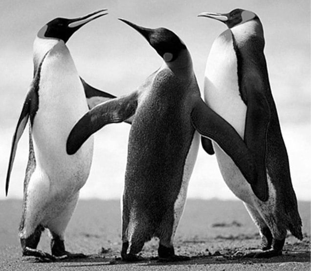
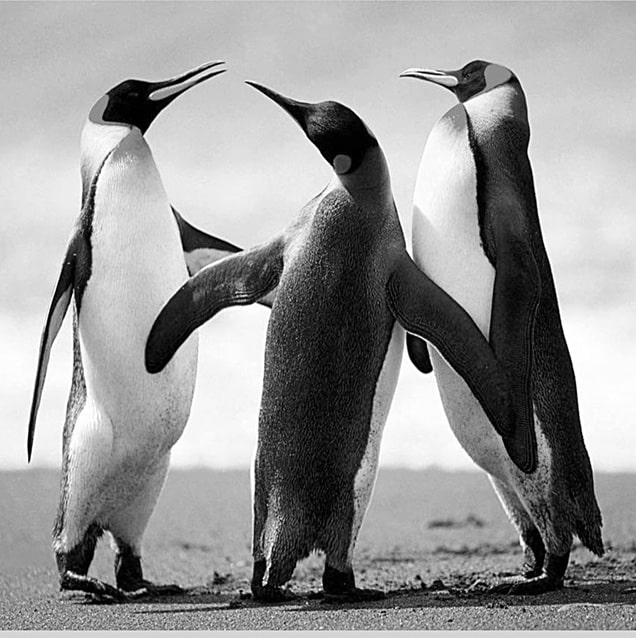
The following set of commands reduces the resolution of image ‘Penguins_grey.jpg’ by half:
A = imread(‘Penguins_grey.jpg’);
A1 = imresize((imresize(A,1/2)),2);
imshow(A1)
Fig. 1 shows image A1.
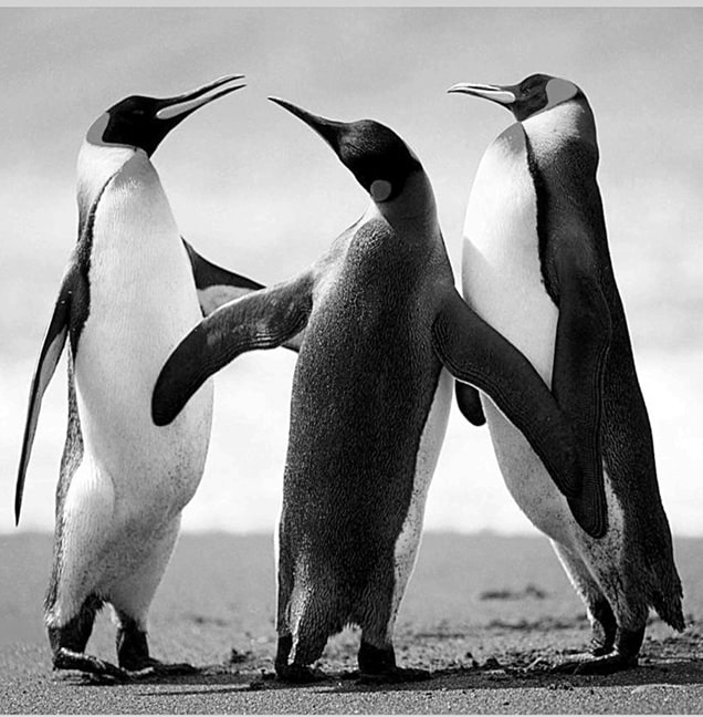
A = imread(‘Penguins_grey.jpg’);
A2 = imresize((imresize(A,1/4)),4);
imshow(A2)
Fig. 2 shows image A2.

A = imread(‘Penguins_grey.jpg’);
A3 = imresize((imresize(A,1/8)),8);
imshow(A3)
Fig. 3 shows image A3.
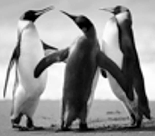
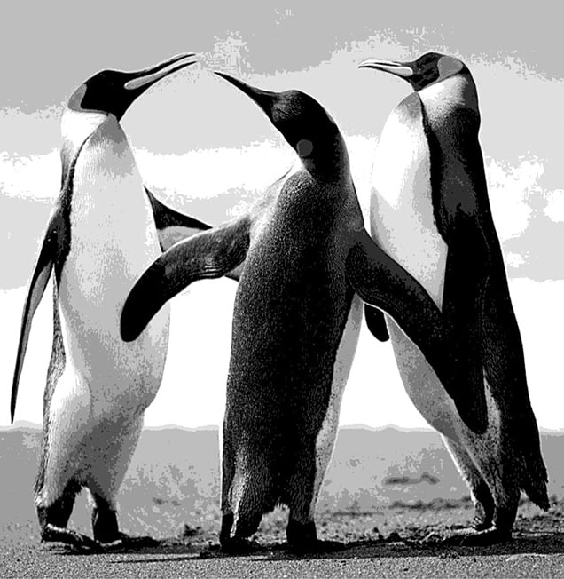
Image quantisation can be described as a mapping process by which groups of datapoints (several pixels within a range of grey values) are mapped to a single point (a single grey level). An image can be re-quantised in MATLAB using the grayslice function. The following set of commands reduces the quantisation levels to 64 and displays the image:
A = imread(‘Penguins_grey.jpg’);
B=grayslice(A,64);
imshow(B,gray(64))
The resultant image of the imshow function is shown in Fig. 4.
The following set of commands reduces quantisation levels to 8 and displays the image:
A = imread(‘Penguins_grey.jpg’);
B=grayslice(A,8);
imshow(B,gray(8))
The resultant image of the imshow function is shown in Fig. 5.
Histogram
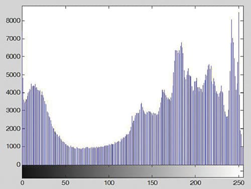
Histogram of a greyscale image represents the frequency of its grey levels occurrence. It is a graph indicating the number of times each grey level occurs in the image. In a dark image, grey levels (and hence the histogram) are cluttered at the lower end. In a uniformly bright image, grey levels (and hence the histogram) are cluttered at the upper end. In a well contrasted image, grey levels (and hence the histogram) would be well spread out over much of the range.
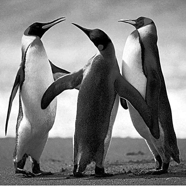
In MATLAB, the histogram can be viewed using the imhist function. As an example, the commands that follow can be used to display the histogram of image Penguins_grey.jpg:
A = imread(‘Penguins_grey.
jpg’);
figure(1), imhist(A);
Fig. 6 shows the histogram generated by the above command.
The three main operations performed on a histogram include histogram stretching, histogram shrinking and histogram sliding. All these operations are described in the following paragraphs.
Histogram stretching
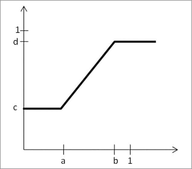
This technique, also known as input cropping, consists of a linear transformation that stretches part of the original histogram so that its non-zero intensity range occupies the full dynamic grey scale.
If the histogram of the image is cluttered at the centre, it can be stretched using imadjust function. The following command stretches the histogram as shown in Fig. 7:
imadjust (F, [a,b], [c,d])
The values of a, b, c and d must be between 0 and 1.
Command imadjust (F, [], [1,0]) inverts the grey value of the image, to produce a result similar to photographic negative.
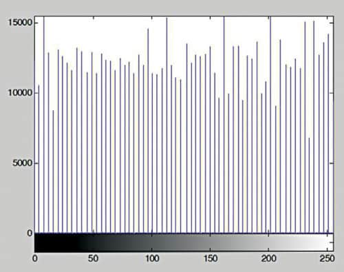
Histogram stretching using above commands requires user input. An alternative approach is to use histogram equalisation command, which is entirely an automatic procedure. Histogram equalisation command in MATLAB is histeq. The use of histeq command is shown below:
A = imread(‘Penguins_grey.jpg’);
HE = histeq(A);
imshow(HE),figure, imhist(HE)
Figs 8 and 9 show the image and the equalised histogram, respectively.
Histogram shrinking
This technique, also known as output cropping, modifies the original histogram such that its dynamic greyscale range is compressed into a narrower greyscale. imadjust function can be used for histogram shrinking.
Histogram sliding
This technique consists of simply adding or subtracting a constant brightness value to all pixels in the image. The overall effect is an image with comparable contrast properties, but higher or lower average brightness, respectively. imadd and imsubtract functions can be used for histogram sliding.
When implementing histogram sliding, you must make sure that pixel values do not go outside the greyscale boundaries. An example of histogram sliding is given below:
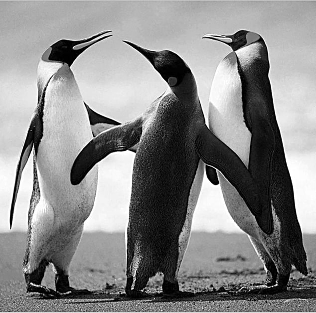
A = imread(‘Penguins_grey.jpg’);
imshow(A),title(‘Original Image’);
B=im2double(A);
bright_add = 0.2;
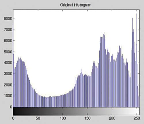
imhist(A), title(‘Original Histogram’);
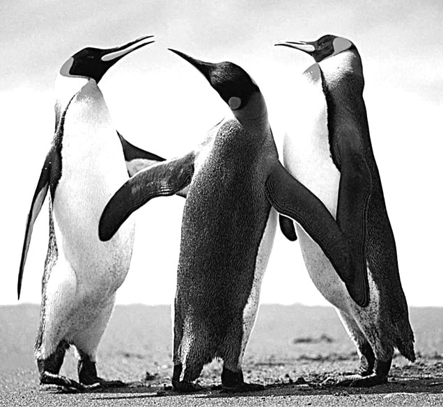
C=B+bright_add;
imshow(C),title(‘New Bright Image’);
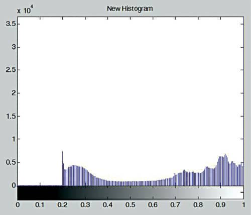
imhist(C), title(‘New Histogram’);
In the example, the image is brightened by adding 0.2 to its pixel values. Figs 10 and 11 show the original image and its histogram, respectively. Figs 12 and 13 show the modified image and its histogram, respectively.
Thresholding
Thresholding is used to remove unnecessary details from an image and concentrate on essentials. It is also used to bring out hidden details, in case the object of interest and background have similar grey levels. Thresholding can be further classified as single thresholding and double thresholding. In MATLAB, single as well as double image thresholding can be done.
Single thresholding
A greyscale image is turned into a binary image (black and white) by first choosing a grey level ‘T’ in the original image, and then turning every pixel black or white depending on whether its grey value is greater than or less than ‘T’. Thresholding is a vital part of image segmentation, where users wish to isolate objects from the background. To convert an image F into black-and-white image G with threshold of 100, the command in MATLAB is G=F>100.
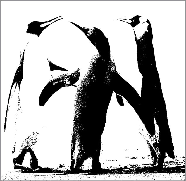
The following example reads image Penguins_grey.jpg and displays both the original image and the image generated after thresholding using a factor of 70:
>>A = imread(‘Penguins_grey.jpg’);
>>imshow(A),figure, imshow(A>70)
Figs 14 and 15 show the original image and the image after thresholding, respectively.
In addition, there is a command in MATLAB which converts a greyscale image or a coloured image into black-and-white image. The command is im2bw(image,level), where image is the greyscale image and level is a value between 0 and 1.
Double thresholding
In this case, there are two values T1 and T2, and the thresholding operation is performed as the pixel becomes white if the grey level is between T1 and T2. Also, the pixel becomes black if the grey level is outside these threshold values.
Image sharpening
Image sharpening is a powerful tool for emphasising texture and drawing viewer focus. It can improve image quality, even more than what is achieved through upgrading to a high-end camera lens.
Most image sharpening software tools work by applying something called an ‘unsharp mask,’ which actually acts to sharpen an image. The tool works by exaggerating the brightness difference along the edges within an image. Note that the sharpening process is not able to reconstruct the ideal image, but it creates the appearance of a more pronounced edge.
The command used for sharpening an image in MATLAB is:
B = imsharpen(A)
It returns an enhanced version of the greyscale or the true-colour (RGB) input image A, where image features such as edges have been sharpened using the unsharp masking method.
B = imsharpen(A, Name, Value,….) sharpens the image using name-value pairs to control aspects of unsharp masking.
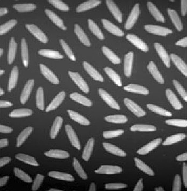
Let us see the use of imsharpen function:
>> a=imread(‘Image_sharpen.jpg’);
>>imshow(a)
Fig. 16 shows the image to be sharpened (Image_sharpen.jpg).
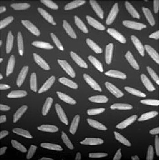
Following commands sharpen the image using the simple imsharpen command:
>> b=imsharpen(a);
>>figure,imshow(b)
Fig. 17 shows the resultant sharpened image.
You can specify ‘radius’ and ‘amount’ parameters in the imsharpen function as given in the example below:
>> b=imsharpen(a,’Radius’,
4,’Amount’,2);
>>figure,imshow(b)
Fig. 18 shows the resultant image.
As you can see, image in Fig. 18 is much sharper than the image in Fig. 17, which, in turn, is much sharper than the image in Fig. 16.
Read Part 3

Where is the next part please ?
You can read part 3 here: https://www.electronicsforu.com/electronics-projects/software-projects-ideas/spatial-filtering-image-processing