


In this series of four articles, fundamentals, as well as advanced topics of image processing using MATLAB, are discussed. The articles cover basic to advanced functions of MATLAB’s image processing toolbox (IPT) and their effects on different images. Part I in this series gives a brief introduction to digital images and MATLAB followed by basic image processing operations in MATLAB including image reading, display and storage back into the disk.
Image processing
Image processing is the technique to convert an image into digital format and perform operations on it to get an enhanced image or extract some useful information from it. Changes that take place in images are usually performed automatically and rely on carefully designed algorithms.
Image processing is a multidisciplinary field, with contributions from different branches of science including mathematics, physics, optical and electrical engineering. Moreover, it overlaps with other areas such as pattern recognition, machine learning, artificial intelligence and human vision research. Different steps involved in image processing include importing the image with an optical scanner or from a digital camera, analysing and manipulating the image (data compression, image enhancement and filtering), and generating the desired output image.

The need to extract information from images and interpret their content has been the driving factor in the development of image processing. Image processing finds use in numerous sectors, including medicine, industry, military, consumer electronics and so on.
In medicine, it is used for diagnostic imaging modalities such as digital radiography, positron emission tomography (PET), computerised axial tomography (CAT), magnetic resonance imaging (MRI) and functional magnetic resonance imaging (fMRI). Industrial applications include manufacturing systems such as safety systems, quality control and automated guided vehicle control.
Complex image processing algorithms are used in applications ranging from detection of soldiers or vehicles, to missile guidance and object recognition and reconnaissance. Biometric techniques including fingerprinting, face, iris and hand recognition are being used extensively in law enforcement and security.
Digital cameras and camcorders, high-definition TVs, monitors, DVD players, personal video recorders and cell phones are popular consumer electronics items using image processing.
MATLAB
MATLAB, an abbreviation for ‘matrix laboratory,’ is a platform for solving mathematical and scientific problems. It is a proprietary programming language developed by MathWorks, allowing matrix manipulations, functions and data plotting, algorithm implementation, user interface creation and interfacing with programs written in programming languages like C, C++, Java and so on.
In MATLAB, the IPT is a collection of functions that extends the capability of the MATLAB numeric computing environment. It provides a comprehensive set of reference-standard algorithms and workflow applications for image processing, analysis, visualisation and algorithm development.
It can be used to perform image segmentation, image enhancement, noise reduction, geometric transformations, image registration and 3D image processing operations. Many of the IPT functions support C/C++ code generation for desktop prototyping and embedded vision system deployment.
What is a digital image?
A digital image may be defined as a two-dimensional function f(x,y), where ‘x’ and ‘y’ are spatial coordinates and the amplitude of ‘f’ at any pair of coordinates is called the intensity of the image at that point. When ‘x,’ ‘y’ and amplitude values of ‘f’ are all finite discrete quantities, the image is referred to as a digital image.
Digitising the coordinate values is referred to as ‘sampling,’ while digitising the amplitude values is called ‘quantisation.’ The result of sampling and quantisation is a matrix of real numbers.
A digitised image is represented as:
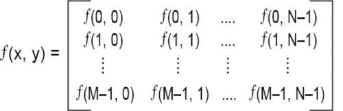
Each element in the array is referred to as a pixel or an image element.
Basic image processing commands in MATLAB
In MATLAB a digital image is represented as:
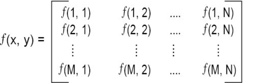
In this representation, you can notice the shift in origin.
Reading images
Images are read in MATLAB environment using the function ‘imread.’ Syntax of imread is:
imread(‘filename’);
where ‘filename’ is a string having the complete name of the image, including its extension.
For example,
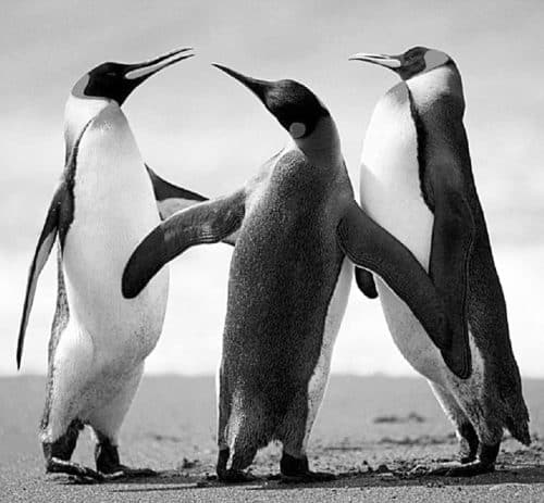
>>F = imread(Penguins_grey.jpg);
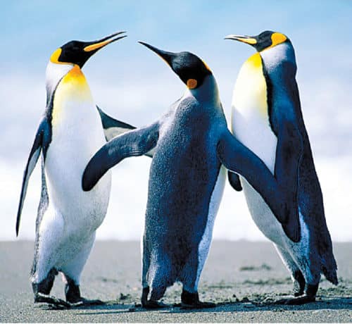
>>G = imread(Penguins_RGB.jpg);
Please note that when no path information is included in ‘filename,’ ‘imread’ reads the file from the current directory. When an image from another directory has to be read, the path of the image has to be specified.
Semicolon (;) at the end of a statement is used to suppress the output. If it is not included, MATLAB displays on the screen the result of the operation specified in that line.
‘>>’ indicates the beginning of a command line as it appears in the MATLAB command window.
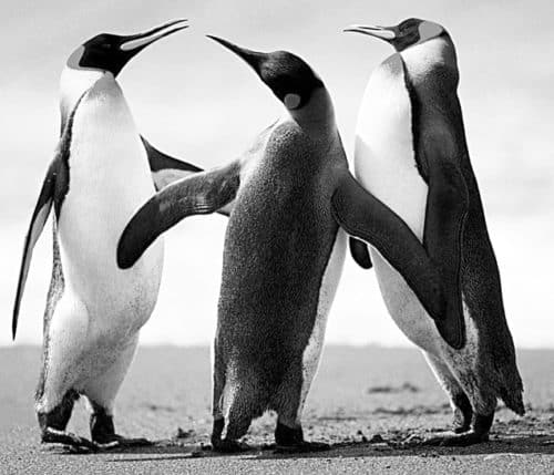
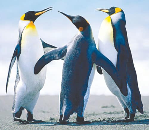
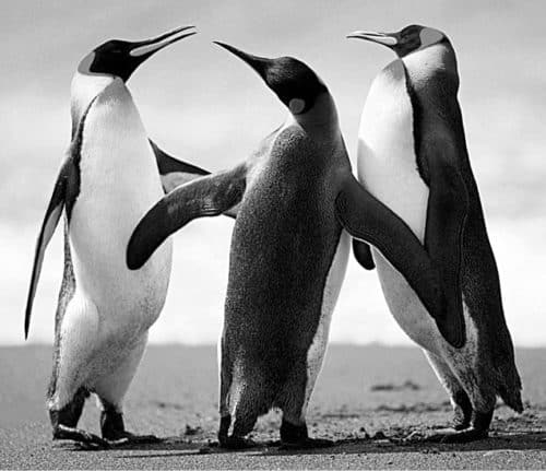
Figs 1 and 2 show grayscale and RGB images of penguins, respectively. These images can be downloaded from the EFY website and stored in the current working directory.
imread, imshow and imwrite functions in MATLAB are used to read images in MATLAB environment, display them on MATLAB desktop and write them to the current directory, respectively
In case of grayscale images, the resultant matrix of the imread statement comprises 256×256 or 65,536 elements. The first statement takes grey values of all the pixels in the grayscale image and puts them into a matrix F(256×256 elements), which is now a MATLAB variable on which various matrix operations can be performed.
In case of RGB images, pixel values now consist of a list of three values, giving red, green and blue components of the colour of the given pixel. Matrix ‘G’ is a three-dimensional matrix 256x256x3. If there is no semicolon, the result of the command is displayed on the screen.
In nutshell, the imread function reads pixel values from an image file and returns a matrix of all pixel values.
To get the size of a 2D image, you can write the command:
[M,N] = size(f)
This syntax returns the number of rows (M) and columns (N) in the image.
You can find additional information about the array using ‘whos’ command.
‘whos f’ gives name, size, bytes, class and attributes of the array ‘f.’
As an example, ‘whos F’ in our case gives:
| Name | Size | Bytes | Class Attributes |
| F | 768×1024×3 | 2359296 | uint8 |
‘whos G’ gives:
| Name | Size | Bytes | Class Attributes |
| G | 768×1024 | 786432 | uint8 |
Image display
Images are displayed on the MATLAB desktop using the function imshow, which has the basic syntax:
imshow(f)
where ‘f’ is an image array of data type ‘uint8’ or double. Data type ‘uint8’ restricts the values of integers between 0 and 255.
It should be remembered that for a matrix of type ‘double,’ the imshow function expects the values to be between 0 and 1, where 0 is displayed as black and 1 as white. Any value between 0 and 1 is displayed as grayscale. Any value greater than 1 is displayed as white, and a value less than zero is displayed as black. To get the values within this range, a division factor can be used. The larger the division factor, the darker will be the image.
As an example, if you give the command imshow(G), the image shown on the desktop is given in Fig. 3. ‘imshow(F)’ displays the image shown in Fig. 4. ‘imshow(f, [low high])’ displays as black all values less than or equal to ‘low’ and as white all values equal to or greater than ‘high.’ The values in between are displayed as intermediate intensity values.
‘imshow(f, [ ])’ sets variable low to the minimum value of array ‘f’ and high to its maximum value. This helps in improving the contrast of images having a low dynamic range.
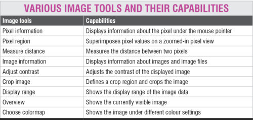
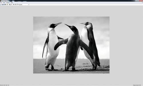
The Image tool in the image processing toolbox provides a more interactive environment for viewing and navigating within images, displaying detailed information about pixel values, measuring distances and other useful operations. To start the image tool, use the imtool function. The following statements read the image Penguins_grey.jpg saved on the desktop and then display it using ‘imtool’:
>>B = imread(Penguins_grey.jpg);
>>imtool(B)
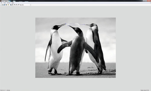
Fig. 5 shows the window that appears when using the image tool. The status text at the bottom of the main window shows the column/row location and the value of the pixel lying under the mouse cursor.
The Measure Distance tool under Tools tab is used to show the distance between the two selected points. Fig. 6 shows the use of this tool to measure distances between the beaks of different penguins.
The Overview tool under Tools tab shows the entire image in a thumbnail view. The Pixel Region tool shows individual pixels from the small square region on the upper right tip, zoomed large enough to see the actual pixel values. Fig. 7 shows the snapshot.

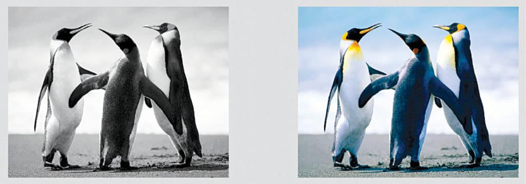
Multiple images can be displayed within one figure using the subplot function. This function has three parameters within the brackets, where the first two parameters specify the number of rows and columns to divide the figure. The third parameter specifies which subdivision to use. For example, subplot(3,2,3) tells MATLAB to divide the figure into three rows and two columns and set the third cell as active. To display the images Penguins_RGB.jpg and Penguins_grey.jpg together in a single figure, you need to give the following commands:
>> A=imread(‘Penguins_grey.jpg’);
>> B=imread(‘Penguins_RGB.jpg’);
>>figure
>>subplot(1,2,1),imshow(A)
>>subplot(1,2,2),imshow(B)
The figure that appears on the screen after the third command is shown in Fig. 8.
Writing images
Images are written to the current directory using the imwrite function, which has the following syntax:
imwrite(f, ‘filename’);
This command writes image data ‘f’ to the file specified by ‘filename’ in your current folder. The imwrite function supports most of the popular graphic file formats including GIF, HDF, JPEG or JPG, PBM, BMP, PGM, PNG, PNM, PPM and TIFF and so on.
The following example writes a 100×100 array of grayscale values to a PNG file named random.png in the current folder:
>> F = rand(100);
>>imwrite(F, ‘random.png’)
When you open the folder in which you are working, an image file named ‘random.png’ is created.
For JPEG images, the imwrite syntax applicable is:
imwrite(f, ‘filename.jpg’, ‘quality’, q)
where ‘q’ is an integer between 0 and 100.
It can be used to reduce the image size. The quality parameter is used as a trade-off between the resulting image’s subjective quality and file size.
You can now read the image Penguins_grey.jpg saved in the current working folder and save it in JPG format with three different quality parameters: 75 (default), 10 (poor quality and small size) and 90 (high quality and large size):
F = imread(‘Penguins_grey.jpg’);
imwrite(F,’Penguins_grey_75.
jpg’,’quality’,75);
imwrite(F,’Penguins_grey_10.
jpg’,’quality’,10);
imwrite(F,’Penguins_grey_90.
jpg’,’quality’,90);
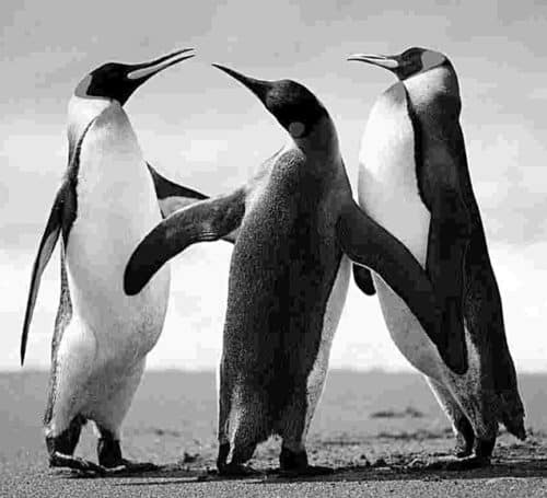
Figs 9 through 11 show images for quality factors of 75, 10 and 90, respectively. You will note that that a low-quality image has a smaller size than a higher-quality image.
The imwrite syntax applicable to TIFF images has the format:
imwrite (g, ‘filename.tif’, ‘compression’,
‘parameter’, ……’resolution’,
[colresrowres])
Image information
File details including file name, data, size, format, height and width can be obtained using the command:
imfinfo’filename’
As an example, the command imfinfo(‘Penguins_grey.jpg’) gives the following information:
ans=
Filename: [1×50 char]
FileModDate: ’02-Aug-2016 09:24:12′
FileSize: 100978
Format: ‘jpg’
FormatVersion: ”
Width: 1024
Height: 768
BitDepth: 8
ColorType: ‘grayscale’
FormatSignature: ”
NumberOfSamples: 1
CodingMethod: ‘Huffman’
CodingProcess: ‘Sequential’
Comment: {}
Information fields displayed by ‘imfinfo’ can be captured into a structural variable that can be used for subsequent computation.
The following example stores all the information into variable ‘K’:
K = imfinfo(‘Penguins_grey.jpg’)
The information generated by ‘imfinfo’ is appended to the structure variable by means of fields, separated from ‘K’ by a dot. As an example, the image height and width are stored in structure fields K.height and K.weight.
Read Part 2
This article was first published on 24 Jan 2018 and was updated on 14 March 2019.
Great explaining especially for beginners .
Thank You for your valuable feedback.
Thank You , it was really helpful.
Is there any such project for audio Processing, Please inform.?
Thank a lot
You are most welcome.
Thank you for briefly explaining for us
You are most welcome!!
very good Work
Thank You for your feedback.
Hello I need to change the background color of the figure when I push any letter ?
Can u help me ?
hi,
for speckle pattern generation how to add gray scale image could you share the code
how can i download the source code?
Hi, the full process of implementing source code is already explained in the article.