


Over the last few decades technology has integrated itself into our daily lives in ways which make us totally reliant on it for our day-to-day tasks. Undoubtedly, technology has only gotten smarter. Considering the trajectory it currently follows, it is only a matter of time until it is able to mimic the way we think and perform our daily tasks. Continue reading to know more.
We are living in an extraordinary time when we are trying to recreate a human brain in machine. Human brain is the most sophisticated organ that nature has given us. Building something which can equal that is a very difficult feat to achieve.

Over the last few years, a lot of studies and findings have been done but that does not seem to be enough by any means. Our limited understanding of this complex organ makes it even harder to mimic all of its functions precisely. Yet, we are determined to make something that can at least be close to the real thing.
Technology landscape
Fig. 1 shows an analogue from the perspective of the technology landscape. It shows that a personal computer and a wired internet connection can be used to connect to the external world.
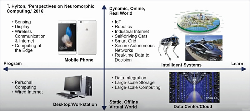
The horizontal dimension in the figure shows that with the help of larger systems we are able to integrate data altogether on a large scale storage and process that data through cloud. The vertical direction contains the devices and technologies that provide a plethora of functionalities.
For example, our cell phones can sense, display, communicate via wireless systems and the internet while providing a great computational power for data processing applications. The computing domain can change from a static and virtual environment to the real world which is highly dynamic in nature. By combining these two dimensions we envision intelligent systems.
Intelligence and artificial intelligence
The concept of intelligence has been discussed by people for many years, even as far back as the 18th century. According to Wilhelm Wundt, “Our mind is so fortunately equipped that it brings us the most important bases for our thought with our having the least knowledge of this work of elaboration.” Clearly, we are curious about intelligence, but we do not know much about our brains and where does it actually come from.
People have become more curious about the intelligence itself through the years of exploration, which has led them to build intelligent systems we today call artificial intelligence (AI). The history of AI can be traced back to a summer workshop back in 1956. It is widely considered as the founding event of AI as a field.
According to Wikipedia, “It is a theory and development of computer systems able to perform tasks normally requiring human intelligence, such as visual perception, speech recognition, decision-making, and translation between languages.”
Evolution of computing power
The chart in Fig. 2 is from Dr Raymond Kurzwell’s book that was published back in 1990, titled “The age of intelligent machines.” This chart summarises the computing power measured as millions of instructions per second. The dots in the chart represent a curve.
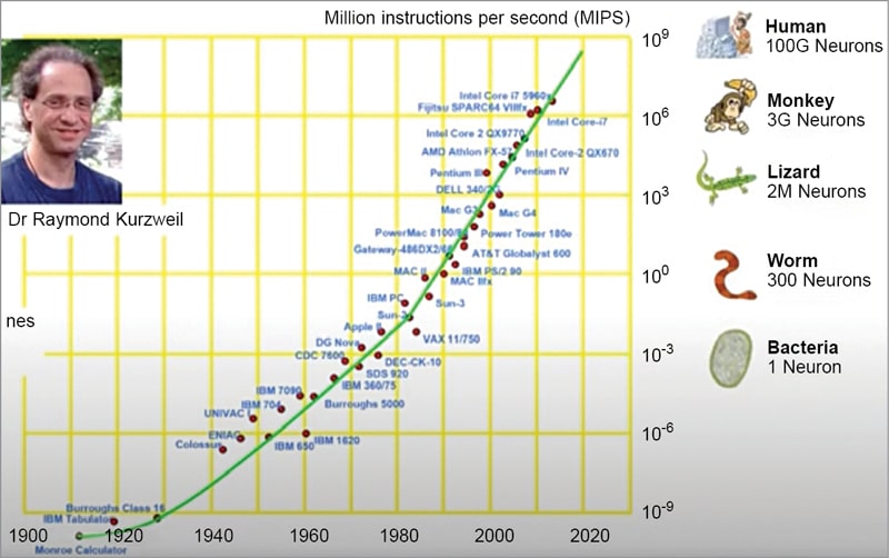
This curve suggested that by the year 2020 the computing power could reach the intelligence level of monkeys and human beings. May be, right now this claim is too bold to go with. But the bottom line is that a sufficiently advanced computer program could exhibit human-level intelligence.
Major limitations
Some limitations have emerged from the intrinsic architecture of the computing system hardware. In the past thirty years, people building computing systems have had different objectives for improving the RAM and processors. They aimed to improve the execution speed for processors while the major goal for the memory part was to increase the storage density. The two components have a huge performance gap to this day.
Another important aspect is the limited power efficiency ceiling. The power efficiency ceiling is much lower than the efficiency provided by human brains. Human brain is indeed the most efficient computing machine there is. So, let us take a quick look at it.
The human brain, on average, contains 15 to 30 billion neurons. It essentially has very complex structures and offers complicated operations. But its power consumption is extremely low at around 20 to 35 volts.
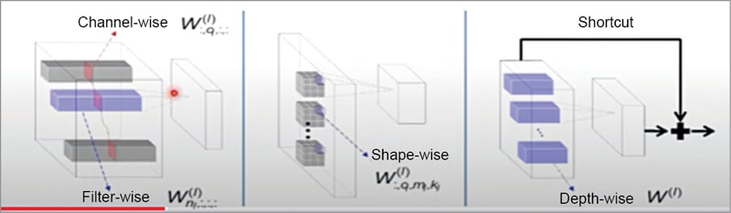
Fig. 3 shows that a human brain contains some gray matter for thinking and white matter for signal transitions. The gray matter consists of a neocortex, which contains six layers where signals travel within the layers. The fundamental elements of the neural cortex are neurons and synapses.
There are three characteristics that can be found in human brain but not in the computers:
Low power consumption
Only about 35 watts of power is consumed by the brain versus roughly 250 watts by a graphics processing unit (GPU) for rigid operations.
Fault tolerance
The cells within the human brains are replaced with new cells as the old ones die. The brain can even heal and continue its functionalities. A silicon based computer system cannot heal itself at all.
Lack of need for the programs
The human brain does not require a program in order to operate as it can learn and unlearn things. This is not the case with a computer.
Let us now look at pruning and sparsification for deep neural networks (DNN) acceleration. Why do we need to sparse DNN models? Some answers are:
- Because the ever-growing size brought challenges to the deployment of the DNN models.
- A lot of studies have shown that the parameters of DNNs are redundant. Many of them can be pruned and reduced so that we can reduce the computation and bandwidth requirement by eliminating that redundancy. This raises the question as to what solution do we have in order to achieve the goal.
When we talk about sparsification and DNNs, there are multiple ways to achieve the goal. We can sparse weight parameters through unstructured prunings or structured prunings. We can also consider activation sparsity where ReLU has been widely adopted.
Our lab has proposed bit-level sparsity, which basically decomposes the weight parameter into binary presentations that aims to remove unwanted zeros from the computation. Then there is inherent sparsity that transposes the convolutions and expands the flick necklace convolutional kernels. Hence, we do not have to involve those zeroes into the computation.
There is a need for structural sparsity because non-structured sparsity may not speedup traditional platforms like GPUs. If we are able to achieve structured sparse state, then we are printing out the weight parameters by rows or columns that will be more friendly to the hardware. These structures can be squeezed into much smaller matrices for the operations. Let us see how we can do that.
Structurally sparse deep neural network
The key idea here is to form a group. A group can be any form of a weight block, depending on what sparse structure you want to learn. For example, in CNNs, a group of weights can be a channel, a 3D filter, a 2D filter, a filter shape fibre (a weight column), and even a layer (in ResNets), as shown in Fig. 3.
Once the groups have been defined, we can apply lasso regulation to the groups. For example, Fig. 4 shows a weight vector with five elements, which we divide into two groups—one with two and the other with three elements.
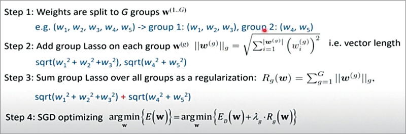
We can apply group lasso on each group by following the equations illustrated in the figure itself. Then we sum the group lasso over all groups as a regulation and add it as a part of the optimisation terms of the overall optimisation objectives. This forms the procedure of our method called the Structure Sparsity Learning.
Sparsity-inducing regulariser for DNN involes the following:
L1 regulariser (sum of absolute values)
- It has been used for sparsity since 1996.
- It is differentiable, convex, and easy to optimise
- It is proportional to the scaling, which will lead to scaling down of all the elements with the same speed, which is undesired
L0 regulariser (number of nonzero values)
- It directly reflects the sparsity by definition
- It is scale invariant. However, our zero regulariser provides no useful gradients
- It needs additional tricks for applying on DNN pruning (stochastic approximation, ADMM), which makes the problem complicated. This leads to certain complexity in the design
Moving beyond lasso
We propose to move beyond L1 and L0 and aim to find the sparsity-inducing regulariser that is both differentiable and scale-invariant for pruning. At this stage the hoyer-square regulariser draws our attention. It is represented by the ratio between the L1 and L2, which is both differentiable and scale-invariant.
For element-wise DNN pruning, we can apply the square version of hoyer regulariser, which has the same range and similar minima structure as L0. We further extend the hoyer-square regulariser to the structure pruning settings.
We can apply hoyer-square regulariser over the L2 norm of each group of weight. The weight within the group can be induced to become zero simultaneously. Let us now look at the effect of the hoyer-square regulariser.
Regulating the activation sparsity:
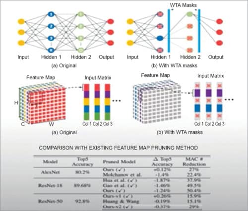
In operations, the activation sparsity is dynamic and the sparsity level is not identical for different inputs. Our group has proposed what is called the Dynamic Winner Takes All (WTA) dropout technique to prune neuron activations layer wise. Hence, the design introduces low overhead for the real-time interface (see Fig. 5).
Mixing precision with bit-level sparsity:
We know that fixed point quantisation is an important model compression technique. In the previous research it was found that some layers can retain higher precision while others can be quantised to less precision. This is the whole idea of mixed precision quantisation.
For a quantised matrix, when the most significant bits of all the elements are zero simultaneously, we can remove the MSB directly (see Fig. 6).

For bit representation we follow the dynamic scaling quantisation procedure. Here (see Fig. 7) we use the element with the largest absolute value in each layer that is the scaling factor and uniformly quantise all the elements to embed the value in binary form.
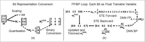
We consider the scaling factor ‘s’ in Ws as an independent trainable variable. This way we are able to enable gradient based training of bit representation. During the training we allow each bit to take a continuous value between zero and two.
Memristor—rebirth of neuromorphic circuits:
ReRam, memristor, or metal-oxide resistive random access memory is essentially for simple two-terminal devices. When we apply voltage or pass current through the devices, their resistance level could change. It is often also called the Programmable Resistance with analogue states.
The spike-based neuromorphic design:
We have moved to spike based neuromorphic design and minimisation of power consumption. It is very similar to the previous structure, but here we use the frequency of the spike to represent the input data amplitude. So, the information is encoded in the spikes instead of analogue voltage. Accordingly, fire circuits are used to produce output spikes along the bit line levels.
We measure the output as impulse number versus the input as the summation of the weighted inputs. The initial expectation was that these will follow a straight line like proportional relations, but the measurements show that it could get saturated. This is mainly because of the operation of the IFC (integrate-and-fire case), which have an upper bound.
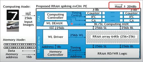
Processing engine with in-situ neuron activation (ISNA):
We integrate 64-kilobit RRAM arrays in this engine. The bottom part of this device is so much like an irregular memory array. On the top part we add our neural processing components (see Fig. 8).
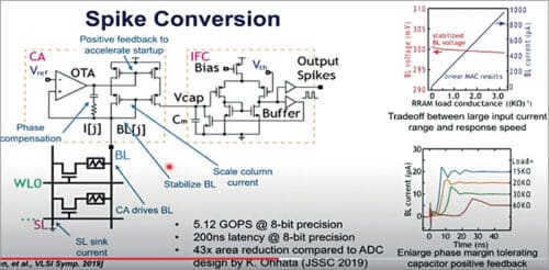
Spike conversion:
The design still uses capacitors to generate spikes. Over here (see Fig. 9), we use the output of the op-amp to form a positive feedback to accelerate the responses from the current amplifier. We use the current mirror to scale down the bit-line current, because in the real network applications, the current can either be several microamperes or several milliamperes—especially at the early stage when the device is not very stable and could result in a larger range of resistance.
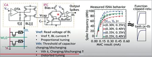
In-situ nonlinear activation function:
In the following design (see Fig. 10) we have two knobs. The reference voltage can control the read voltage of the bit lines while the threshold voltage is used to control the capacitors along with charging and discharging speed. With these distant knobs we are able to slightly tune the shape of neural activation functionalities.
Configurable activation precision:
We measured our chips on the application level and explored trade-offs between high precision weight and activation versus improved performance. Such exploration is useful for system-level, fine-grained optimisation and here are the results.
As mentioned earlier, the designs were fabricated by 150-nanometer complementary metal-oxide semiconductor (CMOS) and HfO RRAM devices. They contain 64-kilobit RRAM devices. The energy efficiency is also high at 0.257 pico joules (pJ/MAC).
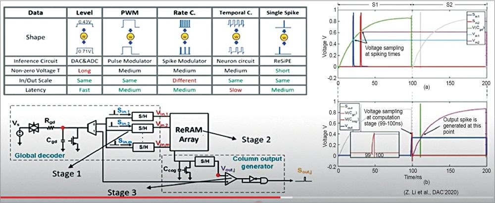
ReRAM based processing engine: ReSiPE
In the last two years we have moved to single spiking designs. The goal is to leverage the timing of the spike for data representation and the matrix operation. For that we divide the design into three stages.
In the first stage we translate the timing of the input spikes to an analogue voltage. Hence, we use a charging process of a capacitor Cgd for reference. When the input spikes ‘S’ then the voltage will be sampled at exactly the spiking time.
In stage two, the hinge signals are fed into the ReRAM crossbar arrays to perform matrix operation and during the computation the capacitor Ccog is charged continuously. The charging speed is determined by the bit-line current.
The last stage is the output stage where Vout is translated to upper spike timing. The voltage of Cgd is again used as the reference and it generates the Vout here (see Fig. 11).
There are three important components that are needed while building machine learning techniques such as data, model, and application. All these elements are connected and operate together. Although we can say that a system is smart, it can still be attacked, hence, further creating a lot of security problems.
Many researchers have shown how well-trained deep learning algorithms can be fooled with adversary tags intentionally. Most of the work focuses on introducing minimal perturbation of the data, which results in a maximally devastating effect on the model. In the case of image based data, it works to disrupt the network’s ability to classify with imperceptible perturbations to the images.
These attacks are of great concern because we do not have a firm understanding of the occurrences taking place inside these interpretable deep models. However, attacks may also provide a way to study the inner workings of such models. There are two types of attacks—the transfer based attacks and activation attacks.
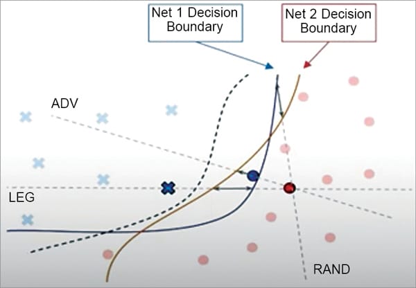
Transfer-based attack:
Fig. 12 shows two different models that are trained with the data from the same distribution. It implies the property of adversarial transferability. This is particularly relevant for a targeted attack. The region for a targeted class in feature space must have the same orientation with respect to the source image for the transferred target to be attacked successfully. In our set-up we train a white box model or source model on the same task as the black box or the target model.
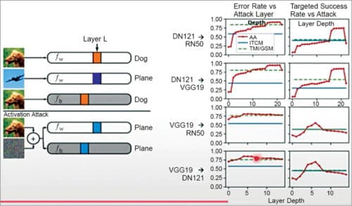
Activation attack:
Here we have designed an activation attack by using the properties of adversarial transferability. As shown in Fig. 13, the white box model (Fw) and a black box model (Fb) are initially correct. We perturb the source image, which drives the layer L activation of the dog image and perturbs the plane image. The results can be seen on the right hand side.
Adversarial vulnerability isolation
To minimise the attack transferability, we studied why attacks even transfer. Inspired by Eli’s paper we found that models entrained on the same data set capture a similar set of non-robust features. These are the features that are highly correlated to the labels yet sensitive to noise. Such features open the door for vulnerabilities and adversary attacks.
We found that a large overlap in the non-robust features leads to overlapping vulnerabilities across different models which, in turn, leads to transferability of the attacks. For every source image and tested set, we randomly sampled another target image and non-robust images that look like the source while having the same hidden features as the target in the hidden layer of the model.
To sum it all up, it is quite understandable that the future computing systems will evolve making them more user-friendly, adaptive, and highly cost-efficient. It is a holistic scheme that integrates the efforts on device, circuit, architecture, system as well as algorithm. To achieve all of this there is a lot of work that needs to be done and a lot of challenges to be met.
This article is based on a tech talk session at VLSI 2022 by Prof. Hai Li (Duke University). It has been transcribed and curated by Laveesh Kocher, a tech enthusiast at EFY with a knack for open source exploration and research.