

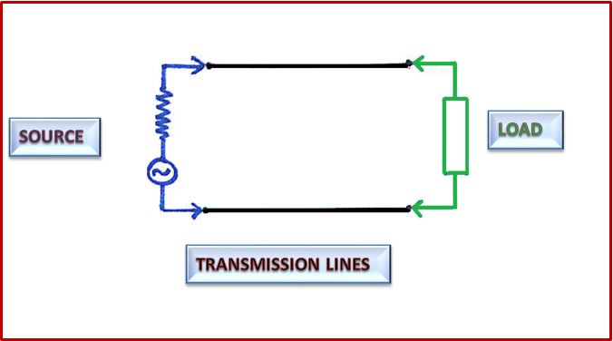
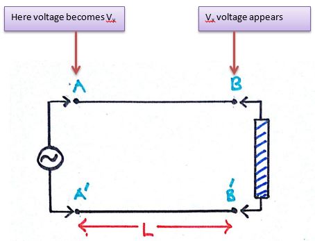
Consider a simple circuit connected to AC source, transmission line and a load. The load may contain the passive components like capacitor, resistor or inductor. Given below is a simple setup that we shall be using for our analysis.

It contains 3 components,
- Source
The source is shown in blue in the figure. It gives sinusoidal input voltage to the circuit of a particular frequency. It has an internal resistance associated with it called source resistance. - Transmission Lines
These are the connecting wires for the current to flow in them. They are shown in black in the figure. - Load
Load is shown in green in the fig. It may contain combination of passive elements like resistor, capacitor or inductor. It’s effective resistance when connected to an AC circuit is called impedance. Load in our daily life are the various appliances running around us like fans, bulbs, refrigerator etc.
The source gives voltage in the sinusoidal form of a particular amplitude and frequency. Keep in mind that sine and cos, both are sinusoidal waves.
Wavelength
Wavelength of the sinusoidal wave is defined as the distance between two successive crest of a wave. It is denoted by ‘Λ’.

Frequency
Frequency is defined as the no of cycles a wave can make in 1 sec. It is measured in Hertz. Following figure shall make our idea more clear about the frequency. It is denoted by ‘f’.
Relation between wavelength and frequency
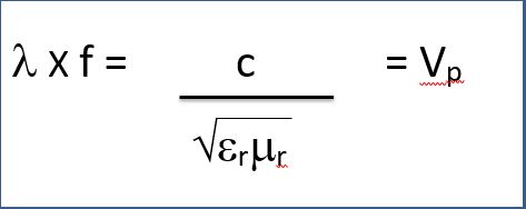
Where;
- Λ = Wavelength
- f = frequency
- c = Speed of light (3 X 10⁸)
- Vp = Phase velocity
- er = Relative permittivity
- ur = Relative permiability
The above relation gives us the relation between the frequency and the wavelength of the input sinusoidal signal. We observe that frequency and wavelength are inversely proportional to each other.
So we define high frequency as follows
When the length of the circuit is comparable to the wavelength of the input sinusoidal wave, then frequency corresponding to that wavelength is considered as high frequency.
We shall now look into the concept of transit time effect.
Transit Time Effect
Consider a simple circuit connected to AC source, transmission line and a load.
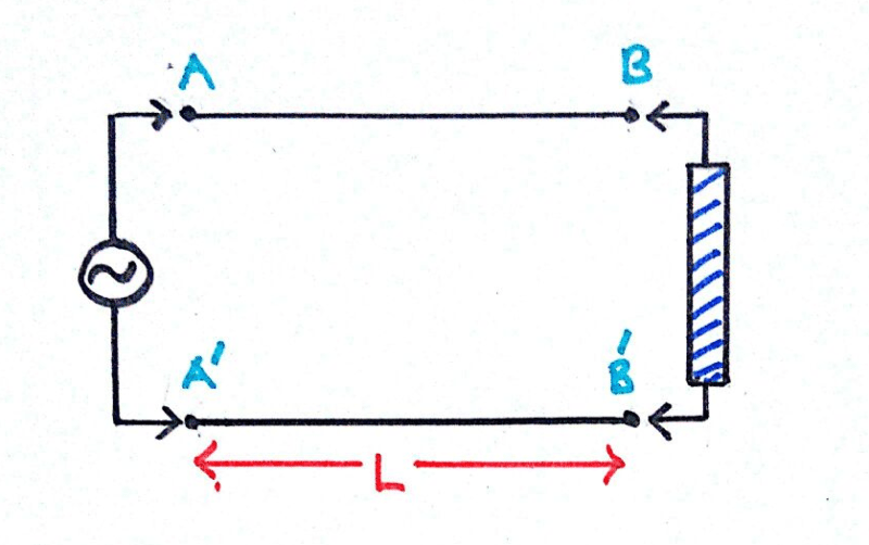
We apply a sinusoidal voltage of frequency ‘f’ and hence time period 1/f.
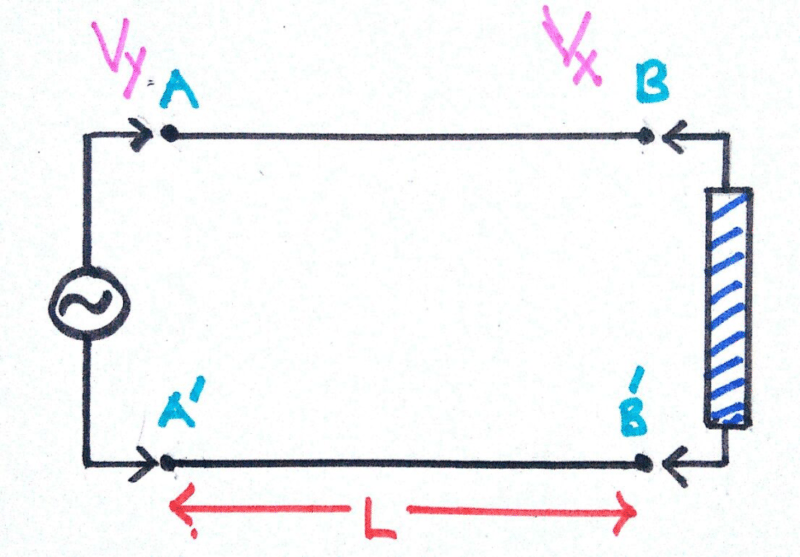
Let at some instant of time the voltage across AA’ is Vx. It is a fact that no signal can travel with infinite speed in a physical system. Hence this voltage Vx does not occur at BB’ at the same instant. It will appear at BB’ after some finite delay of time. This finite delay is called transit time of the signal for the length of the line i.e. time taken for the voltage applied at one end to appear at the other end.
Transit time is given by;
tr = L/v
Where :
- tr = Transit Time
- L= Length of the conductor (Transmission line)
- V= Velocity
Thus the transit time is the time after which the voltage at A appears at B.
At t=0;
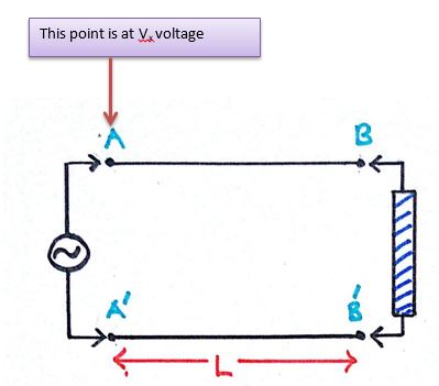
When this voltage appears at BB’, the voltage at AA’ does does not remain Vx as it was varying with time. Let us assume it becomes Vy.
At t= tr (Transit time)
Thus a potential difference is developed between the points A and B. No matter how small the length of the conducting wire, some amount of potential drop will always be there. This is called the transit time effect.
The transit time effect can be neglected if the potential drop between A and B is very small. The transit time effect can be neglected if the potential drop between A and B is very small. So essentially what we say is that if the Transit time is much smaller compared to the time period of the signal then the transit time effects can be neglected.
However when the Transit time becomes comparable to the period of the signal then we have to incorporate the effect of the Transit time. Thus we see that now to perform circuit analysis the size of the structure or space has started playing a significant role. Observations made;
- At High frequency
The time period of input voltage becomes small, so the transit time becomes comparable to T. So the transit time effects cannot be neglected. Without consideration of transit time effect, our analysis will be inaccurate. - At Low frequency
The time period of the input voltage becomes large and transit time is negligible compared to time period. Hence the transit time effects can be neglected. We have seen that to ignore the transit time effect input voltage time period must be greater than transit time.
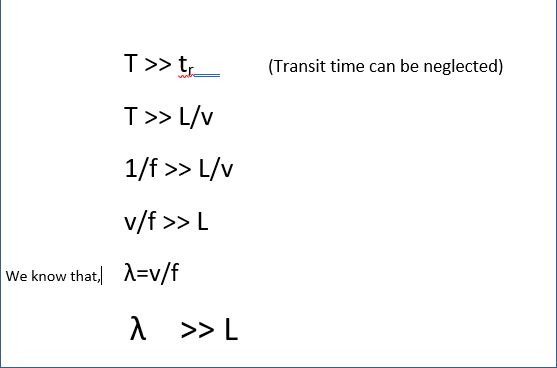
Hence we see that to neglect the transit time effect the wavelength of the input voltage must be larger than length of the conducting wires. When the wavelength is large the frequency is small. When the length of the conducting wires becomes comparable to the wavelength of the input voltage then the transit time effects cannot be neglected. The wavelength is small i.e comparable to length of the conducting wire and hence the frequency corresponding to it is very high. This frequency is called High Frequency.
Hence we conclude that the frequency of the input AC voltage source is considered high when the wavelength at that frequency is comparable to the length of the conducting wires. This is the situation where current and voltage laws cannot be applied directly. We shall now look at it with an example;
We consider a situation where the length of the transmission line (conducting wire) is 1.5 cm.
Case 1
Applied frequency (f)=1 MHz = 106 v= speed of light = 3×10⁸
Thus λ = v/f = 9486 cm = 94.86 m4
The wavelength is larger than the length of the transmission line (1.5 cm)
Case 2
Applied frequency (f)= 10 GHz =1010 Hz
Thus λ = v/f = 0.9486 cm
Here the wavelength is smaller than the transmission line (1.5 cm). Hence the applied frequency is considered as high frequency.
Skin effect
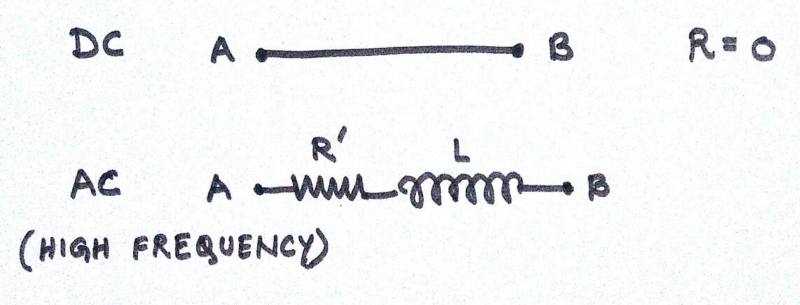
A piece of wire when used in circuits at DC voltage is considered as short circuit. This is because at DC input, the distribution of current is uniformly distributed over its cross sectional area. At high frequency, the current does not flow through the core, rather it flows through the sides of the wire. Higher is the frequency more the current flows through the skin.
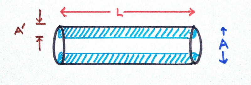
Thus the effective area where the current is flowing is reduced. This is called skin effect. We know that resistance is given by:
R=rl/A
Where
- R= Resistance
- r= resistivity of the wire
- L= length of the conducting wire
- A= Cross sectional area of wire
Thus we see that resistance is inversely proportional to cross sectional area. So as the effective are gets reduced the resistance of the wire increases and the wire can no longer be considered as short circuited.
Behavior of passive components at high frequency
When AC current flows through a wire there is a magnetic field associated with it. This magnetic field linked with the current gives inductor like behavior. Also due to skin effect there is some resistance. Hence at high frequency a conductor behaves as an inductance with a series resistance.
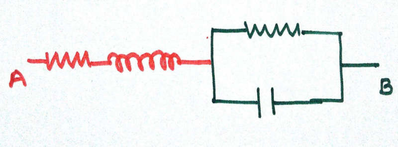
The capacitor along with its lead can be considered as a combination of inductor, resistor and a capacitor. The resistance and inductor are due to the leads of the capacitor. The resistance in parallel with the capacitor is due to the insulation/ internal resistance of the capacitor.
Inductive reactance for inductor;
Xl = 2Pf L
Capacitive reactance for capacitor;
Xc = 1 / 2Pf C
Hence as the frequency increases the inductor dominates. Hence overall circuit becomes inductive. The capacitor at high frequency starts behaving like an inductor.
Consider 2 points A and B on the inductor. They are at different potentials. Also the region between them is filled with air which is a dielectric. Hence the overall setup is analogous to parallel plate capacitor. Hence the inductor at high frequency can be assumed as a series resistance and inductor having a capacitor in parallel.
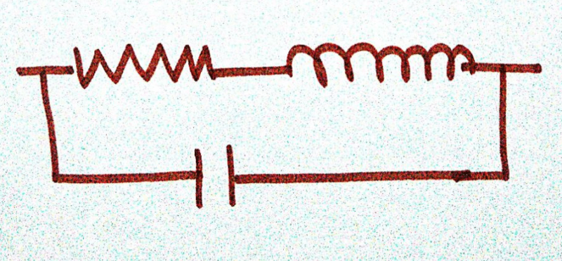
In this setup at high frequency capacitive behaviour dominates (Since capacitive reactive becomes small and capacitor is in parallel). Thus at high frequency the inductor behaves as a capacitor.
Feel interested? Check out the learning corner for more interesting articles.