


Read Part 2
Spatial filtering techniques refer to those operations where the resulting value of a pixel at a given coordinate is a function of the original pixel value at that point as well as the original pixel value of some of its neighbours. These operations are classified into linear filtering operations and non-linear filtering operations.
In linear filters, the resulting output pixel is computed as a sum of products of the pixel values and mask coefficients in the pixel’s neighbourhood in the original image. In other words, if the function by which the new grey value is calculated is a linear function of all the grey values in the mask, then the filter is referred to as a linear filter. Mean filter is an example of linear filter.
In non-linear filters, the resulting output pixel is selected from an ordered sequence of pixel values in the pixel’s neighbourhood in the original image. Median filter is an example of non-linear filter.

Linear filters
Convolution and correlation are the two fundamental mathematical operations involved in linear filters based on neighbourhood-oriented image processing algorithms.
Convolution
Convolution processes an image by computing, for each pixel, a weighted sum of the values of that pixel and its neighbours. Depending on the choice of weights, a wide variety of image processing operations can be implemented.

Different convolution masks produce different results when applied to the same input image. These operations are referred to as filtering operations and the masks as spatial filters. Spatial filters are often named based on their behaviour in the spatial frequency. Low-pass filters (LPFs) are those spatial filters whose effect on the output image is equivalent to attenuating the high-frequency components (fine details in the image) and preserving the low-frequency components (coarser details and homogeneous areas in the image). These filters are typically used to either blur an image or reduce the amount of noise present in the image. Linear low-pass filters can be implemented using 2D convolution masks with non-negative coefficients.
High-pass filters (HPFs) work in a complementary way to LPFs, that is, these preserve or enhance high-frequency components with the possible side-effect of enhancing noisy pixels as well. High-frequency components include fine details, points, lines and edges. In other words, these highlight transitions in intensity within the image.
There are two in-built functions in MATLAB’s Image Processing Toolbox (IPT) that can be used to implement 2D convolution: conv2 and filter2.
conv2 computes 2D convolution between two matrices. For example, C=conv2(A,B) computes the two-dimensional convolution of matrices A and B. If one of these matrices describes a two-dimensional finite impulse response (FIR) filter, the other matrix is filtered in two dimensions.
filter2 function rotates the convolution mask, that is, 2D FIR filter, by 180° in each direction to create a convolution kernel and then calls conv2 to perform the convolution operation.
Y=filter2(h,X) filters the data in ‘X’ with the two-dimensional FIR filter in the matrix ‘h.’ It computes the result ‘Y’ using two-dimensional correlation, and returns the central part of the correlation that is of the same size as ‘X.’
Y=filter2(h,X,shape) returns the part of ‘Y’ specified by the shape parameter. Shape is a string with one of these values:
1. ‘full’ returns the full two-dimensional correlation. In this case, ‘Y’ is larger than ‘X.’
2. ‘same’ (default) returns the central part of the correlation. In this case, ‘Y’ is of the same size as ‘X.’
3. ‘valid’ returns only those parts of the correlation that are computed without zero-padded edges. In this case, ‘Y’ is smaller than ‘X.’
There is no single best approach to use the filter2 function. However, the method is dictated by the problem at hand.
One can create filter by hand or by using the fspecial function. fspecial is an IPT function designed to simplify the creation of common 2D image filters. Its syntax is:
h = fspecial(type, parameters)
where:
1. ‘h’ is the filter mask
2. ‘type’ is one of these: ‘average’—averaging filter, ‘disk’—circular averaging filter, ‘gaussian’—Gaussian low-pass filter, ‘laplacian’—2D Laplacian operator, ‘log’—Laplacian of Gaussian (LoG) filter, ‘motion’—approximates the linear motion of a camera, ‘prewitt’ and ‘sobel’—horizontal edge-emphasising filters, ‘unsharp’—unsharp contrast-enhancement filter)
3. ‘parameters’ are optional and vary depending on the type of filter; for example, mask size, standard deviation (for ‘gaussian’ filter) and so on
imfilter is another command for implementing linear filters in MATLAB.
The syntax for imfilter is:
g = imfilter(f, h, mode, boundary_
options, size_options);
Where ‘f’ is the input image, ‘h’ is the filter mask, and ‘mode’ can be either ‘conv’ or ‘corr,’ indicating whether filtering will be done using convolution or correlation (which is the default), respectively.
boundary_options refer to how the filtering algorithm should treat border values. There are four possibilities:
1. X. The boundaries of the input array (image) are extended by padding with a value ‘X.’ This is the default option (with X=0).
2. ‘symmetric’. The boundaries of the input array (image) are extended by mirror-reflecting the image across its border.
3. ‘replicate’. The boundaries of the input array (image) are extended by replicating the values nearest to the image border.
4. ‘circular’. The boundaries of the input array (image) are extended by implicitly assuming the input array is periodic, that is, treating the image as one period of a 2D periodic function.
As regards size_options, there are two size options for the resulting image: ‘full’ (output image is the full filtered result, that is, the size of the extended/padded image) or ‘same’ (output image is of the same size as input image), which is the default.
‘g’ is the output image.
Correlation. Correlation is the same as convolution without mirroring (flipping) of the mask before the sums of products are computed. The difference between using correlation and convolution in 2D neighbourhood processing operations is often irrelevant because many popular masks used in image processing are symmetrical around the origin.
Linear low-pass filters
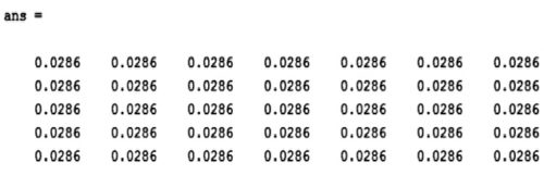
The averaging filter is a linear LPF implemented using ‘average’ option in the fspecial function. The command given below produces an averaging filter of size 5×7:
fspecial(‘average’, [5,7])
The output of this command in MATLAB is:
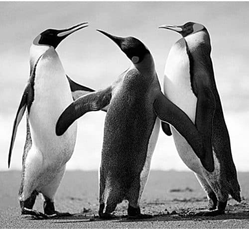
The code given below applies an averaging filter of dimensions 3×3 to the image Penguins_grey.jpg:
A = imread(‘Penguins_grey.jpg’);
B = fspecial(‘average’);
C = filter2(B,A);
figure, imshow(A),figure, imshow(C/255)
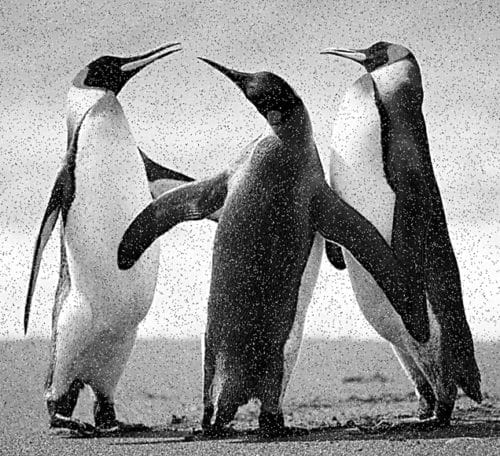
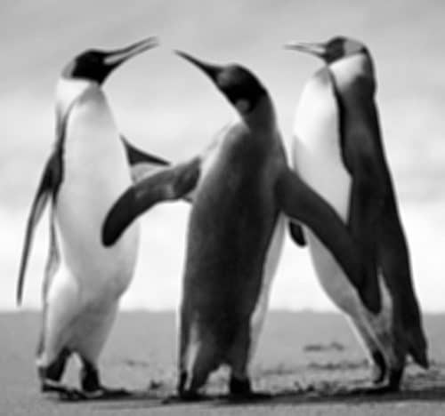
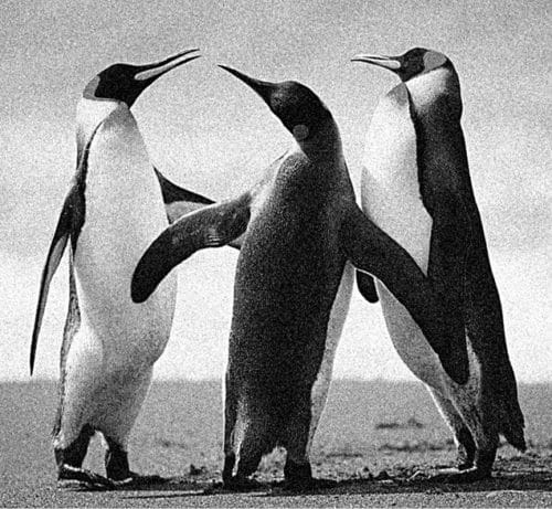
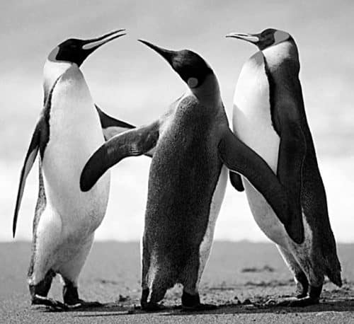
Matrix B is a 3×3 matrix with each matrix element having a value of 0.111. Matrix C has data of type ‘double.’ We can divide it by 255 to obtain a matrix with values in the 0-1 range for use with imshow function. Both the original image and the filtered image are shown in Figs 1 and 2, respectively.
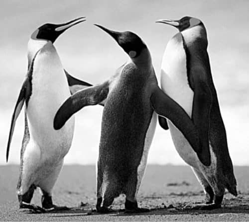
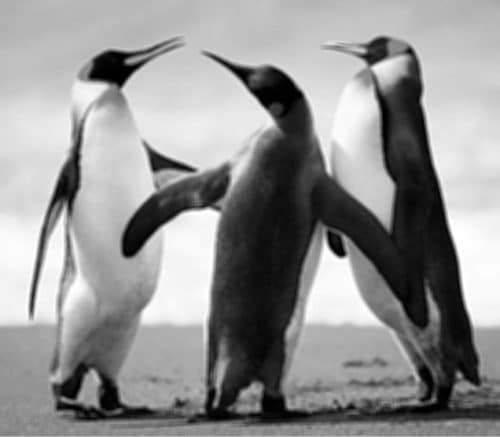
As you can see from the filtered image, the averaging filter blurs the image and the edges in the image are less distinct than in the original image. Larger the size of the averaging filter, more is the blurring effect. The code given below shows the averaging filter operation using an average filter of 9×9:
A = imread(‘Penguins_grey.jpg’);
B = fspecial(‘average’,[9,9]);
C = filter2(B,A);
figure, imshow(A),figure, imshow(C/255)
Fig. 3 shows the filtered image.
Averaging filter is an arithmetic mean filter. Other types of mean filters include geometric mean filters, harmonic mean filters and contra-harmonic mean filters. Mean filter is the simplest and the most widely used spatial smoothing filter.
The averaging filter operates on an mxn sliding window by calculating the average of all pixel values within the window and replacing the centre pixel value in the destination image with the result.
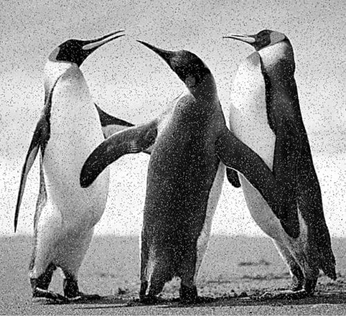
As mentioned above, the averaging filter causes the blurring effect in the image, proportional to the window size. This helps in reduction of noise, especially Gaussian or uniform noise. As an example, let us add salt and pepper noise to the Penguins_grey.jpg image and filter it using the averaging filter. Salt and pepper noise causes very bright (salt) and very dark (pepper) isolated spots in an image.
The command for adding salt and pepper noise to an image is:
A = imread(‘Penguins_grey.jpg’);
Noise_snp=imnoise(A,’salt & pepper’);
imshow(Noise_snp)
Fig. 4 shows the Penguins_grey.jpg image with salt and pepper noise added.
Following commands remove the salt and pepper noise from Fig. 4:
>> B = fspecial(‘average’, [9,9]);
>> C = filter2(B,Noise_snp);
>>imshow(C/255)
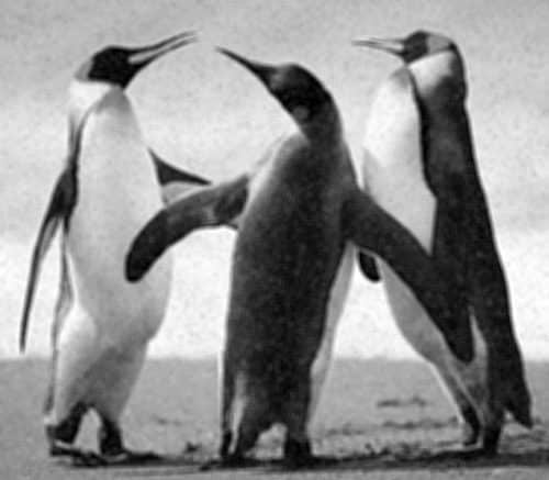
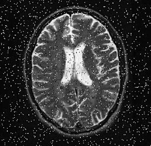
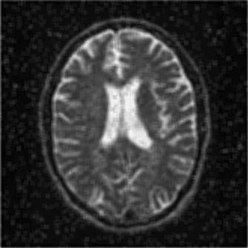
Fig. 5 shows the resultant image. As you can see, the image in Fig. 5 is blurred but the salt and pepper noise has been removed. Fig. 6 shows another image (MRI image) with salt and pepper noise and Fig. 7 shows the image after performing the following operations:
>> a=imread(‘MRI_snp.jpg’);
>>imshow(a)
>> B = fspecial(‘average’, [9,9]);
>> C = filter2(B,a);
>>imshow(C/255)
A variation of the arithmetic mean filter is the geometric mean filter. It is primarily used on images with Gaussian noise. This filter is known to retain image detail better than the arithmetic mean filter.
Gaussian filters are another type of linear filter. These are low-pass filters, based on the Gaussian probability distribution function as given below:
ƒ(x)=e–x2/2σ2
where ‘σ’ is the standard deviation.
Gaussian filters have a blurring effect which looks very similar to that produced by neighbourhood averaging.
The following commands apply Gaussian filter to the image Penguins_grey.jpg:
>> A = imread(‘Penguins_grey.jpg’);
>> G1=fspecial(‘gaussian’,[11,11]);
>> G1image=filter2(G1,A)/256;
>>imshow(G1image)
The numbers within the square brackets give the size of the filter, the default value of which is 3×3. The final parameter is the standard deviation. If any value is not specified, a default value of 0.5 is assumed. In the command given above, since the standard deviation parameter is not specified, default value of 0.5 is taken.
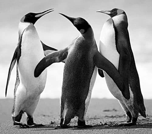
Fig. 8 shows a Gaussian filtered image with standard deviation value taken as 0.5.
When the standard deviation is specified to be 5, as shown in the command (G1=fspecial(‘gaussian’,[11,11],5);), the resultant image is as shown in Fig. 9.
Linear high-pass filters
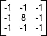
Linear HPFs can be implemented using 2D convolution masks with positive and negative coefficients, which correspond to a digital approximation of the Laplacian—a simple, isotropic (rotation-invariant) second-order derivative that is capable of responding to intensity transitions in any direction.
An alternative digital implementation of the Laplacian takes into account all eight neighbours of the reference pixel in the input image and can be implemented by the convolution mask given below:
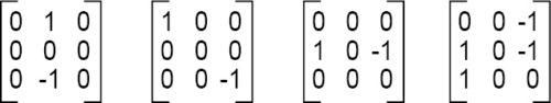
Directional difference filters
Directional difference filters are similar to the Laplacian high-frequency filter but emphasise edges in a specific direction. There filters are usually called emboss filters. There are four representative masks that can be used to implement the emboss effect:
Linear high-pass filters include Prewitt and Sobel operators. These are also referred to as first-order edge-detection methods. High-pass filters are used for edge detection and edge enhancement operations.
The IPT function edge has options for both Prewitt and Sobel operators. Edge detection using Prewitt and Sobel operators can also be achieved by using imfilter command with the corresponding 3×3 masks (which can be created using fspecial command).
Following code extracts edges in the image using Prewitt operator:
>> A = imread(‘Penguins_grey.jpg’);
>>Prewitt_A=edge(A,’Prewitt’);
>>imshow(Prewitt_A)
Fig. 10 shows the resultant image.
Let us now add Gaussian noise to the Penguins_grey.jpg image. We then process it using the Prewitt edge detector:
>> A = imread(‘Penguins_grey.jpg’);
>>A_noise=imnoise(A,’gaussian’);
>>Prewitt_A_noise=edge(A_noise,
’Prewitt’);
>>imshow(A_noise)
>>imshow(Prewitt_A_noise)
Fig. 11 shows the image with the added Gaussian noise and Fig. 12 shows the image filtered with Prewitt edge detector.
Following code shows the use of Sobel operator for edge detection:
>> A = imread(‘Penguins_grey.jpg’);
>>Sobel_A=edge(A,’sobel’);
>>imshow(Sobel_A)
Fig. 13 shows the resultant image.
Let us now add Gaussian noise to the Penguins_grey.jpg image. We then process it using the Sobel edge detector:
>> A = imread(‘Penguins_grey.jpg’);
>>A_noise=imnoise(A,’gaussian’);
>>Sobel_A=edge(A,’sobel’);
>>imshow(Sobel_A)
Fig. 14 shows the resultant image.
Non-linear filters
Non-linear filters work at a neighbourhood level, but do not process pixel values using the convolution operator. Instead, these usually apply a ranking (sorting) function to pixel values within the neighbourhood and select a value from the sorted list. For this reason, these are sometimes called rank filters. Examples of non-linear filters include median filter and max and min filters.
Median filter is a popular non-linear filter used in image processing. It works by sorting the pixel values within a neighbourhood, finding the median value, and replacing the original pixel value with the median of that neighbourhood. Median filter works much better than an averaging filter with comparable neighbourhood size in reducing salt and pepper noise. Because of its popularity, median filter has its own function (medfilt2) provided by the IPT.
Following code shows the use of median filter to remove salt and pepper noise from the image Penguins_grey.jpg:
A = imread(‘Penguins_grey.jpg’);
Noise_snp=imnoise(A,’salt& pepper’);
imshow(Noise_snp)
Filtered_snp=medfilt2(Noise_snp,[3 3]);
imshow(Filtered_snp)
Figs 15 and 16 show noisy and cleaned images, respectively. Fig. 17 shows another noisy image and Fig. 18 shows this image cleaned using median filter.
Sliding window operations
Sliding window neighbourhood operations are implemented in the IPT using one of these two functions: nlfilter or colfilt. Both functions accept a user-defined function as a parameter. Such function can perform linear as well as non-linear operations on the pixels within a window. For rank filters, the IPT function ordfilt2 makes it very easy to create min, max and median filters.
The syntax for nlfilter has three arguments: the image matrix, the size of the filter and the function to be applied. The following line defines a filter that takes the maximum value in a 3×3 neighbourhood:
cmax = nlfilter(c,[3,3],‘max(x(:))’);
A filter that takes minimum value in a 3×3 neighbourhood is defined by the following command:
cmin = nlfilter(c,[3,3],‘min(x(:))’);
Region of interest processing
Filtering operations are sometimes performed only in a small part of an image, referred to as the region of interest (ROI). ROI is specified by defining a mask that limits the portion of the image in which the operation will take place.
Image masking is the process of extracting a sub-image from a larger image for further processing. ROI processing can be implemented in MATLAB using a combination of two functions: roipoly (for image masking) and roifilt2 (for actual processing of the selected ROI).

where is part 4?
Thank you for your comment. We have updated the article with 4th part link. You can access the 4th article here.