





Electronic colour matching makes it possible to create new colours from existing colour materials with greater accuracy and consistency. Colours are widely used in textiles, beverages, medical tablets, paints, automobiles, plastics, and household appliances, where new shades are often developed through trial-and-error mixing. This project presents a scientific method for electronic colour matching using the TI 3200 colour sensor and MATLAB to formulate novel colours. The technique makes it possible to produce customised shades, such as a pinkish yellow for beverages or a bluish-green tint for vehicles, with improved precision. This work is based on extensive research in colour science and technology and was also presented at the International ACHMEA Congress in 2018.
Three things are to be learnt in this process.
- The colour representation CIE Chromaticity chart
- The Color sensor Arduino based unit was published in EFY 2017.
- The following is the list of available colour materials.
List of Available Colour Materials
The following colour materials are available for the colour-mixing experiments.
Colouring Agents
- Alizarin C
- Reactive Red M-2BE
- Acid Red 337
- Disperse Red 13
- Acid Red 119
- D&C Red No. 34
- Solvent Red 8
- Acid Red 4
- Acid Red 88
- Red BLI
- Reactive Bright Red K2G
- Alizarin Yellow R
- Basic Yellow 11
- C.I. Acid Yellow 9
- C.I. Reactive Yellow 145
- C.I. Vat Yellow 1
- Naphthol Blue Black
- Acid Orange 24
- Acid Blue 92
- Reactive Blue
Food Colouring Agents
A growing number of natural food colourings are being commercially produced, partly due to consumer concerns surrounding synthetic colourings. Some examples include:
- Caramel colouring, made from caramelized sugar, used in cola products and also in cosmetics.
- Annatto, a reddish-orange dye made from the seed of the Achiote.
- A green dye made from chlorella algae.
- Cochineal, a red dye derived from the cochineal insect, Dactylopius coccus.
- Betanin extracted from beets.
- Turmeric
- Saffron
- Paprika
- Elderberry
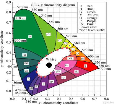
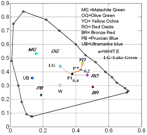
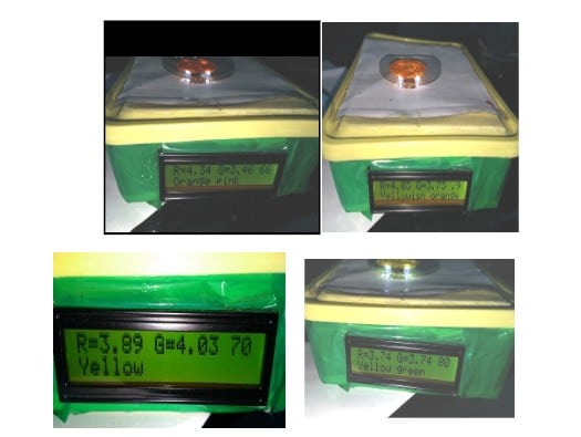
Fig. 3(a) shows the colour of a yellow ochre pigment, which appears orange-pink. Its R and G coordinates are 4.34 and 3.46, respectively. When approximately 10% lemon yellow pigment (R = 3.74 and G = 3.74) was added, the colour changed to a yellowish orange, as shown in Fig. 3(b). Taking the yellow pigment shown in Fig. 3(c) as the starting colour, the addition of a small amount of sap green pigment changed the colour to yellow-green, as shown in Fig. 3(d).
Then using colour conversion commands, the RGB values can be converted to the xyz format and from that to the chroma, luminance xyl format. The xy values of this result is the point we need on the chromaticity chart
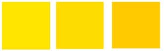
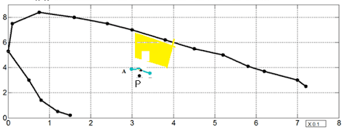
- On the computer, simulate the required colour by entering RGB values in the 0-1 range and using the image formation code, show the image on the monitor (Fig. 5 (a)). (Appendix 4.1 gives the image formation code).
- On the computer, to show the colours of the nearest available pigments: First apply the A pigment on the glass plate and take the reading with the instrument. This gives the x,y,l values. These values are multiplied values by 10. After dividing by 10, the values are entered in the program (App.2) to find their colours (Fig. 5 (b) and Fig. 5 (c)).
- Mix colours A, B in proportions of 4:1,3::1,2:1 and 1:1. The mixes must be independent and one should not use the 4:1 mixture itself to adjust to 3:1 or 2:1. The instrument reading is taken for all these. The xy co-ordinates are plotted on the chroma chart outline. The Chroma chart outline is plotted using the code given in Appendix 4.3.
- Then, after noting the values of the mix data points, they can be plotted on the chroma chart outline as shown in Fig. 6. That is shown as the blue green line. The point of the required colour shown in Fig. 5 (a) is P.
- Then, we find the proportion of the mix from the blue green path’s points. The points of the mix ratios will not be linear in general. Only an estimate of the proportion can be made from these points.
So, it is then required to select two coloured pigments whose chroma values are around the point. Then, we experiment with the instrument for mixing these two colours in several proportions; mixing is done on a glass plate with a spatula and examined for uniformity with a lens. Then we could plot the chroma values of the points as a locus joining the two chroma points of the two pigments. It may be that the required colour is obtained from the locus or is quite near to it with a difference of <0.01 in both x and y values. The mix ratio of the two pigments is then determined.
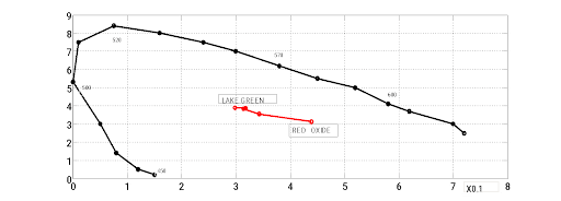
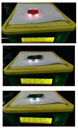
It is better to choose two coloured pigments whose x,y values are close by on the chart. In the Fig. 6 below, The two coloured paints which are in the yellow green and green regions are chosen and mixed in 3:1,3:2 and 3:1 proportions. Then using the instrument (fig. Photo) the r,g values and also their hue values are found immediately as and when they are mixed. The values are noted down and used to plot on the chromaticity chart. Using Matlab, the required colour’s point can be calculated.
Three points combination for colour mixing
If the colour required cannot be met by two pigments available and if the locus of their mixing departs from the co-ordinates of the needed colour, then we can select three colours which are in the vicinity of the required colour. Then, experiments are done using any two colours at a time and drawing the paths of their loci. A triangular shape is within which our needed chroma point is.
After drawing the three loci, the nearest distance of the point of the required mix is found to the three loci. Since the locus is a curve, the minimum distance can be found by a search calculation on the locus or by an approximation with a straight line for the curve.
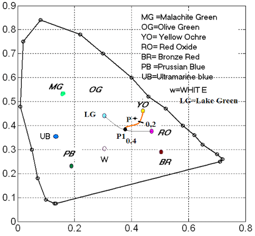
Knowing which locus is nearest, then we find that near point on the locus and estimate the mix proportion for it. For example, if the point is at the 40% mix or near position, (shown as P1), then a mix of pigments of this ratio is prepared and applied uniformly on the glass plate.
Then, commencing with this, little by little, we add the third pigment (YO). This third pigment is the pigment not included in the mix on the plate.
As we add proportions of the third colour pigment and find the r,g values, the path of that locus is determined (red colour curve shown). That locus would pass very near to the required colour point P. The proportions of mix of the first two pigments along with the third pigment (0.2 for ratio of P1 to YO), which gives this nearness to the required colour are noted. The procedure is illustrated in Fig. 7. The mix is in the ratio 1:0.4:0.2 for RO, LG and YO pigments.
A formula can be worked out on the basis of the above experiments.
Finding the minimal distance among three colours
In order to get a colour point other than available colours (vide Appendix 4.4), one has to choose at least three colours A,B,C which are having their co-ordinates close to the point. Out of the set of N colours we take the first three lowest values, after sorting them in accordance with their distances to the required colour point.
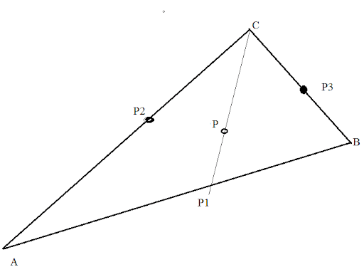
The three points will form a triangle and it is usual to show this as what is called ‘colour Gamut’. It may be possible to get a colour point within this triangle using these colours. The procedure for mixing using such three colours has been outlined above. That will use the instrument developed or a colorimeter to plot the three curves of mixing A to B, B to C and C to A.
Thus, unlike what is usually shown in colour gamuts, the three points join by curves and not straight lines. The proportions of the mixes can be indicated on the curves roughly. Then, the nearest point on that curve is taken and is combined with the third colour and it may pass close to the required colour.
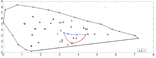
The three colours nearest to the point only will provide the required colour and it is not possible to choose three distant colours to get to the point P. For instance in the previous figure, we may not use points such as A1, B1 and C1 to bring the mixture to point P. That is because the paths of colour mixing may not be steady enough for long distances among the points and there might be variations in the mix at different samplings.
Thus, having determined the minimal distance points A, B and C, we may combine them optimally. For that purpose, we may arrive at a mix of (A_B)C or (B_C)A or (C_A)B. If the costs of the products A, B and C are known, then the total cost of the mixed colour will be dependent on the proportions of A:B:C. Since the paths are nonlinear, the combinations of first A and B and then with C will not be same as the combination of first B and C and then A.
Finding the cost of pigment mixing
If all the pigments A, B and C are equal in cost, then the geometric calculation itself will give the cheapest choice. For this the calculation is just to drop a line to the side AB from point P and then add the distance from P1 to the nearer of the two ends of that side. The cost value is just proportional to the length AP1+P1P or BP1+P1P, the lesser one being considered. Similar possibilities are CP2+P2P and CP3+P3P. The least of these is a choice. Suppose CP2+P2P is the least, then we mix C with the proportion CP2/CB of B; and add P2P/P2A of A. The ratio of mixing A,B,C is P2P/P2A:CP2/CB:1.
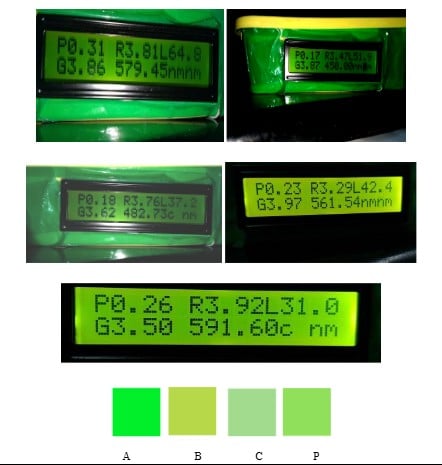
Colours of pigments of coordinates A,B,C are to be used to mix and get a new colour P. The experiments on the mixing and the data noted on the measurement unit are given in Fig. 10 (a) to (f) below.
The following program gives the code for showing an image for a chosen R,G,B values
for j=1:128;
for k=1:128S(j,k,:)=rgba;end
end
imshow(S)
Program to convert the instrument readings to rgb colour and plot the image.
C= makecform('xyl2xyz');
C1= makecform('xyz2srgb');
xa= [2.95 3.4 0.7];
xyza= applycform(xa,C); % first convert the 3D xyz format.
rgba=applycform(xyza,C1); % finds r,g,b values form xyz format
for j=1:128
for k=1:128
S(j,k,:)=rgba;  %Use 128 x 128 pixels to show the colour square
end
end
figure; imshow(S)
This program plots the chroma chart outline.
a=[1.5, .2;1.2,.5; .8 1.4;.5 3; 0 5.3;0.1 7.5;0.75 8.4;1.6 8; 2.4 7.5; 3 7;3.8 6.2;4.5 5.5;5.2 5; 5.8 4.1; 6.2 3.7;7 3; 7.2 2.5; ]
x1=a(:,1)
y1=a(:,2)
plot(x1,y1,'-o')
axis([0 8 0 9])
holdon
The following program calculates the data using Fig.1 for three colour mixtures to white to plot the graph shown in Fig. 8.
% distance,co-ord. r and co-ord g
feo=[0,0,0; 10,0.06,0;40,0.12,-0.02;100,0.151,-0.032]
x=feo(:,1);
y1=feo(:,2);
%plot(x',y')
y2=feo(:,3);
d=sqrt(y1.*y1+y2.*y2);
plot(x',d','-bs','LineWidth',2)
hold on
% y=feo(:,3)
%hold on;y=feo(:,3);plot(x,y,'r')
prblu=[0,0,0;1,-0.04,-0.04;10,-0.08,-0.14;40,-0.06,-0.185;100,-0.1,-0.2]
x=prblu(:,1);
y1=prblu(:,2);
y2=prblu(:,3);
d=sqrt(y1.*y1+y2.*y2);
plot(x',d','-bs','LineWidth',2)
holdon%subplot(111)
%y=prblu(:,3);
%plot(x,y,'r')
bro_Red=[0,0,0;1,-0.02,-0.01;10,0,-0.1;32,0.1,-0.1; 100,0.15,-0.08]
%subplot(111)
x=bro_Red(:,1);y1=bro_Red(:,2);y2=bro_Red(:,3);
%plot(x,y);hold on; plot(x,y1,'r')
d=sqrt(y1.*y1+y2.*y2);
plot(x',d','--o','LineWidth',2)
The following program plots the Chromaticity chart and shows the paths of the colour mixing from data on paths collected by the instrument.
a=[1.5, .2;1.2,.5; .8 1.4;.5 3; 0 5.3;0.1 7.5;0.75 8.4;1.6 8; 2.4 7.5; 3 7;3.8 6.2;4.5 5.5;5.2 5; 5.8 4.1; 6.2 3.7;7 3; 7.2 2.5;]
x1=a(:,1)
y1=a(:,2)
plot(x1,y1,'-o')
axis([0 8 0 9])
hold on
%green to red
g2r=[2.98,3.88;3.18, 3.86;3.14,3.84;3.43,3.55]
% red to blue
r2b=[4.39,3.12; 3.92,3.13;3.44,3.28;3.23,3.44]
% blue to green
b2g=[2.89,3.47;3.25,3.81;3.13,3.88;3.11,3.91]
   x1=r2b(:,1);y1=r2b(:,2);
    plot(x1,y1,'-o')
keyboard
x1=g2r(:,1);y1=g2r(:,2);
    plot(x1,y1,'-o')
   keyboard
    x1=r2b(:,1);y1=r2b(:,2);
plot(x1,y1,’-os’)
    keyboard
    x1=b2g(:,1);y1=b2g(:,2);
   plot(x1,y1,'-og')
Conclusion
Although the toolbox may appear difficult to understand initially, once users become familiar with it, they can easily develop colour mixtures optimised for cost, toxicity, or other desired parameters using the available colours to create new and interesting colour combinations.
Authors-
K. Padmanabhan, R. C. Nayar, S. Anathi and A. Deepa
1. Prof. Rtd. Instrumentation, Univ. Madras
2. Prof. Rtd. Textiles Tech, A. C. Tech, Ana Univ.
3. Prof. Rtd. Instrumentation and I. T., Madras Univ.
4. Prof. Electronics, A. K. Bakthavatsalam Institute of Science, Univ. Madras