


Convolutional neural networks (CNNs or ConvNets) used in machine learning are similar to neural networks. These are made up of neurons that have learnable weights and biases. Each neuron receives some inputs, performs a dot product and optionally follows it with a non-linearity. The whole network expresses a single differentiable score function from the raw image pixels on one end to class scores at the other, with a loss function (such as support vector machine/softmax) on the last (fully-connected) layer. Softmax function is just a generalisation of logistic function. It is used as a cost function for probabilistic multi-class classification, and by itself it is not a classifier.
CNNs have revolutionised the pattern-recognition computation process. Prior to the widespread adoption of CNNs, most pattern-recognition tasks involved hand-crafted features extraction followed by classification. With CNNs, features are now learned automatically from training examples. The CNN approach is especially powerful when applied to image recognition because convolution operation captures the 2D nature of images. By using the convolution kernels to scan an entire image, relatively few parameters need to be learned compared to the total number of operations.

CNN architecture
Unlike a regular neural network, the layers in a CNN have neurons arranged in three dimensions: width, height and depth. Here, ‘depth’ refers to the third dimension of an activation volume, not to the depth of a full neural network, which can refer to the total number of layers in a network.
For example, input images in CIFAR-10 are an input volume of activations, and the volume has dimensions 32x32x3 (width, height and depth, respectively). Neurons in a layer will only be connected to a small region of the layer before it, instead of all of the neurons in a fully-connected manner. Moreover, the final output layer for CIFAR-10 would have dimensions 1x1x10, because by the end of the ConvNet architecture the full image will reduce into a single vector of class scores, arranged along the depth dimension.
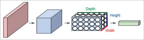

Fig. 1: Illustration of a ConvNet
Every layer of a CNN transforms the 3D input volume to a 3D output volume of neuron activations. In the example shown in Fig. 1, the red input layer holds the image, so its width and height would be image dimensions, and the depth would be 3 (red, green, blue channels).
Typically, CNN architectures comprise three types of layers stacked together: convolutional layer, pooling layer and fully-connected (FC) layer.
A simple ConvNet for CIFAR-10 classification has the architecture
Input->Conv->Relu->Pool->FC as detailed below:
1. Input [32x32x3] holds the raw pixel values of the image; in this case, an image of width 32 and height 32, with three colour channels R, G and B
2. Conv layer computes the output of neurons that are connected to local regions in the input, each computing a dot product between their weights and a small region they are connected to in the input volume. This may result in a volume such as [32x32x12] if twelve filters are used
3. Relu layer applies an element-wise activation function, such as the max(0,x) thresholding at zero. This leaves the size of the volume unchanged ([32x32x12]).
4. Pool layer performs a down-sampling operation along the spatial dimensions (width, height), resulting in a volume such as [16x16x12]
5. Fully-connected (FC) layer computes class scores, resulting in a volume of size [1x1x10], where each of the ten numbers correspond to a class score, such as among the ten categories of CIFAR-10. Each neuron in this layer is connected to all the numbers in the previous volume.
Thus, CNNs transform the original image layer by layer from the original pixel values to the final class scores. Note that some layers contain parameters, while others don’t. In particular, Conv/FC layers perform transformations that are a function of not only activations in the input volume but also of neuron parameters (weights and biases). On the other hand, Relu/Pool layers implement a fixed function. Parameters in Conv/FC layers are trained with gradient descent so that class scores computed by the CNN are consistent with labels in the training set for each image.
Architecture for vehicle control
In end-to-end learning system for self-driving cars, weights of the network are trained to minimise the mean-squared error between the steering command output by the network and the command of either the human driver or the adjusted steering command for off-centre and rotated images. Fig. 2 shows the network architecture for vehicle control, which consists of nine layers, including a normalisation layer, five convolutional layers and three fully connected layers.
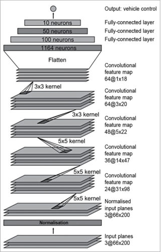
Fig. 2: CNN architecture for vehicle control
The input image is split into YUV planes and passed to the network. The network has about 27 million connections and 250,000 parameters. The first layer of the network performs image normalisation; the normaliser is hard-coded and not adjusted in the learning process. Performing normalisation in the network allows the normalisation scheme to be altered with the network architecture, and accelerated via GPU processing.
The convolutional layers are designed to perform feature extraction, and are chosen empirically through a series of experiments that vary layer configurations. This model uses strided convolutions in the first three convolutional layers with a 2×2 stride and a 5×5 kernel, and a non-strided convolution with a 3×3 kernel size in the final two convolutional layers. The five convolutional layers are followed with three fully connected layers, leading to a final output control value which is the inverse-turning-radius. The fully connected layers are designed to function as a controller for steering, but by training the system end-to-end, it is not possible to make a clean break between which parts of the network function primarily as feature extractor, and which serve as controller.
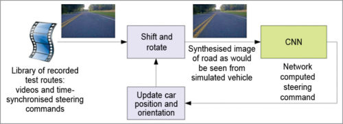
Fig. 3: Drive simulator
Training and simulator
The first step in training a neural network is to select the frames for use. The collected data is labeled with road type, weather condition and the driver’s activity (staying in a lane, switching lanes, turning and so forth). To train a CNN to do lane following, data is selected where the driver is staying in a lane, while the rest is discarded.
Then, the video is sampled at a rate of 10 frames per second because a higher sampling rate would include images that are highly similar, and thus not provide much additional useful information. To remove a bias towards driving straight, the training data includes a higher proportion of frames that represent road curves.
After selecting the final set of frames, the data is augmented by adding artificial shifts and rotations to teach the network how to recover from a poor position or orientation. The magnitude of these perturbations is chosen randomly from a normal distribution. The distribution has zero mean, and the standard deviation is twice the standard deviation that is measured with human drivers. Artificially augmenting the data does add undesirable artifacts as the magnitude increases.
Fig. 4 shows a screenshot of the simulator in interactive mode. The simulator takes prerecorded videos from a forward-facing on-board camera connected to a human-driven data-collection vehicle, and generates images that approximate what would appear if the CNN were instead steering the vehicle. These test videos are time-synchronised with the recorded steering commands generated by the human driver. Since human drivers don’t drive in the centre of the lane all the time, there is a need to manually calibrate the lane’s centre as it is associated with each frame in the video used by the simulator.
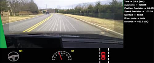
Fig. 4: Simulator in interactive mode
The simulator transforms the original images to account for departures from the ground truth. Note that this transformation also includes any discrepancy between the human driven path and the ground truth. The transformation is accomplished by the same methods. The simulator accesses the recorded test video along with the synchronised steering commands that occurred when the video was captured. The simulator sends the first frame of the chosen test video, adjusted for any departures from the ground truth, to the input of the trained CNN, which then returns a steering command for that frame.
The CNN steering commands as well as the recorded human-driver commands are fed into the dynamic model of the vehicle to update the position and orientation of the simulated vehicle. In Fig. 4, the green area on the left is unknown because of the viewpoint transformation. The highlighted wide rectangle below the horizon is the area which is sent to the CNN.
The simulator then modifies the next frame in the test video so that the image appears as if the vehicle was at the position that resulted by following steering commands from the CNN. This new image is then fed to the CNN and the process repeats. The simulator records the off-centre distance (distance from the car to the lane centre), the yaw, and the distance travelled by the virtual car. When the off-centre distance exceeds one metre, a virtual human intervention is triggered, and the virtual vehicle position and orientation is reset to match the ground truth of the corresponding frame of the original test video.
Fig. 5 shows how the CNN learns to detect useful road features on its own, with only the human steering angle as training signal. It was not explicitly trained to detect road outlines. CNNs are able to learn the entire task of lane and road following without manual decomposition into road or lane marking detection, semantic abstraction, path planning and control. A small amount of training data from less than a hundred hours of driving is sufficient to train the car to operate in diverse conditions, on highways, local and residential roads in sunny, cloudy and rainy conditions.
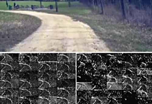
Fig. 5: How the CNN sees an unpaved road. Top: Camera image sent to the CNN; bottom left: activation of the first-layer feature maps; bottom right: activation of the second-layer feature maps
Image identification in autonomous vehicles
To be able to identify images, autonomous vehicles need to process a full 360-degree dynamic environment. This creates the need for dual-frame processing because collected frames must be combined and considered in context with each other. A vehicle can be equipped with a rotating camera to collect all relevant driving data. The machine must be able to recognise metric, symbolic and conceptual knowledge as demonstrated in Fig. 6.
Metric knowledge is the identification of the geometry of static and dynamic objects, which is required to keep the vehicle in its lane and at a safe distance from other vehicles. Symbolic knowledge allows the vehicle to classify lanes and conform to basic rules of the road. Conceptual knowledge allows the vehicle to understand relationships between traffic participants and anticipate the evolution of the driving scene. Conceptual knowledge is the most important aspect for being able to detect specific objects and avoid collisions.
One current method of obstacle detection in autonomous vehicles is the use of detectors and sets of appearance-based parameters. The first step in this method is the selection of areas of interest. This process narrows down areas of the field of vision that contain potential obstacles.
Appearance cues are used by the detectors to find areas of interest. These appearance cues analyse two-dimensional data and may be sensitive to symmetry, shadows, or local texture and colour gradients. Three-dimensional analysis of scene geometry provides greater classification of areas of interest. These additional cues include disparity, optical flow and clustering techniques.
Disparity is the pixel difference for an object from frame to frame. If you look at an object alternately closing one eye after the other, the ‘jumping’ you see in the object is the disparity. It can be used to detect and reconstruct arbitrarily shaped objects in the field.
Optical flow combines scene geometry and motion. It samples the environment and analyses images to determine the motion of objects. Finally, clustering techniques group image regions with similar motion vectors as these areas are likely to contain the same object. A combination of these cues is used to locate all areas of interest.
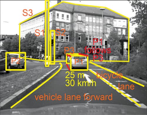
Fig. 6: Image identification in autonomous vehicles
While any combination of cues is attainable, it is necessary to include both appearance cues and three-dimensional cues as the accuracy of three-dimensional cues decreases quadratically with increasing distance. In addition, only persistent detections are flagged as obstacles so as to lower the rate of false alarms.
After areas of interest have been identified, these must be classified by passing them through many filters that search for characteristic features of on-road objects. This method takes a large amount of computation and time. The use of CNNs can increase the efficiency of this detection process. CNN-based detection system can classify areas that contain any type of obstacle. Motion-based methods such as optical flow heavily rely on the identification of feature points, which are often misclassified or not present in the image.
All the knowledge-based methods are for special obstacles (pedestrians, cars, etc) or in special environments (flat road, obstacles differing in appearance from ground). Convolutional neural networks are the most promising for classifying complex scenes because these closely mimic the structure and classification abilities of the human brain. Obstacle detection is only one important part of avoiding a collision. It is also vital for the vehicle to recognise how far away the obstacles are located in relation to its own physical boundaries.
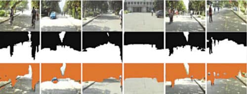
Fig. 7: Obstacle detection test results: Input images (top), ground truths with black as positive (middle) and detected obstacles with orange as positive (bottom)
Depth estimation
Depth estimation is an important consideration in autonomous driving as it ensures the safety of passengers as well as other vehicles. Estimating the distance between an obstacle and the vehicle is an important safety concern.
A CNN may be used for this task as CNNs are a viable method to estimate depth in an image. In a study, researchers trained their network on a large dataset of object scans, which is a public database of over ten thousand scans of everyday 3D objects, focused on images of chairs and used two different loss functions for training. They found that bi-weight trained network was more accurate at finding depth than the L2 norm. With images of varying size and resolution, it had an accuracy between 0.8283 and 0.9720 with a perfect accuracy being 1.0.
While estimating depth on single-frame stationary objects is simpler than on moving objects seen by vehicles, researchers found that CNNs can also be used for depth estimation in driving scenes. They fed detected obstacle blocks to a second CNN programmed to find depth. The blocks were split into strips parallel to the lower image boundary. These strips were weighted with depth codes from bottom to top with the notion that closer objects would normally appear closer to the lower bound of the image. The depth codes went from ‘1’ to ‘6’ with ‘1’ representing the most shallow areas and ‘6’ representing the deepest areas. The obstacle blocks were assigned the depth code for the strip they appeared in.
The CNN then used feature extraction in each block area to determine whether vertically adjacent blocks belonged to the same obstacle. If the blocks were determined to be the same obstacle, they were assigned the lower depth code to alert the vehicle of the closest part of the obstacle. CNN was trained on image block pairs to develop a base for detecting depth and then tested on street images as in the obstacle detection method. The CNN had an accuracy of 91.46 per cent in two-block identification.