


 Amplitude modulation (AM) is a signal modulation technique that is widely used by radio stations for transmitting their programs. This project proposes a Python GUI-based Amplitude Modulation simulator to study AM.
A user can vary various parameters—such as modulation index, amplitude and frequency of the modulating signal, and carrier signal—and observe the output. The project can be used to simulate the signal modulation by radio engineers for designing different carrier signals and their modulation and demodulation.
| Bill of Material | ||
| Components | Quantity | Description |
| Raspberry Pi | 1 | Raspberry Pi board to connect LCD |
| LCD | 1 | For display |
| 5V, 2A power adaptor | 1 | For power supply |
For amplitude modulation, the carrier waveform is modulated according to the instantaneous amplitude of the message (baseband) signal. To understand, let us consider a sinusoidal wave as the message signal that needs to be transmitted. Let us say, the amplitude of the message signal is Am and its frequency is fm. The mathematical time-domain representation of the message signal would be:
m(t) = Am.cos (2πƒmt) ........Eq 1
The carrier signal is a high-frequency radio wave with amplitude Ac and frequency fc, which is represented by:
c(t) = Ac.cos (2πƒct) ........Eq 2
The equation of modulated waveform is:
The modulation index defines modulation level, which can be defined as:
![]()
Software Installation
The software required for the project is Python 3.10.1, Tkinter, Matplotlib, and NumPy.
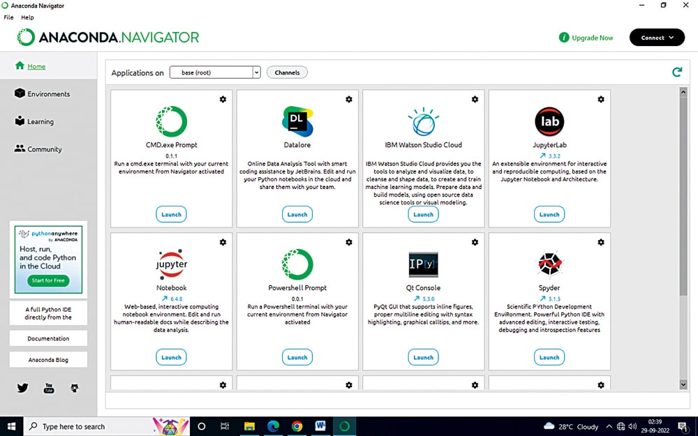
First, install the Anaconda Distribution or Python 3 environment in Raspberry Pi. Then install Tkinter, Matplotlib, and NumPy.
Next, import these libraries into the code and prepare the code for the signal modulator simulator.
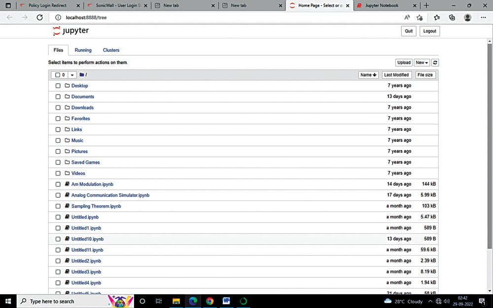
Jupyter Notebook from Anaconda creates an interactive web-based Python computing environment in any browser that is selected while installation.
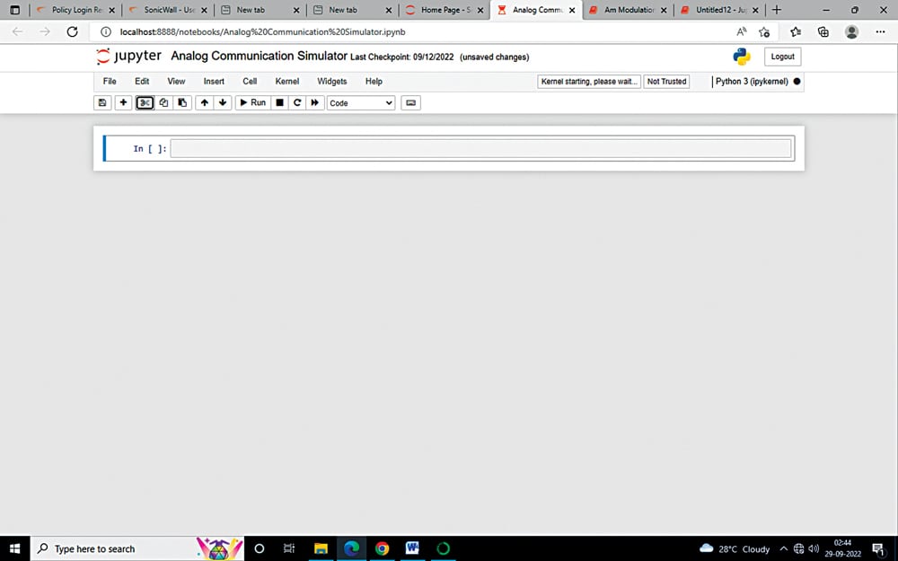
Create a new notebook from the file menu of Jupyter IDE by selecting Python 3 as ipykernal. Rename the new notebook as Analog Communication Simulator.
This project uses functions from Tkinter, Matplotlib, and NumPy libraries, hence import their libraries. You can use pip install and conda install to install the libraries. For example, pip install matplot
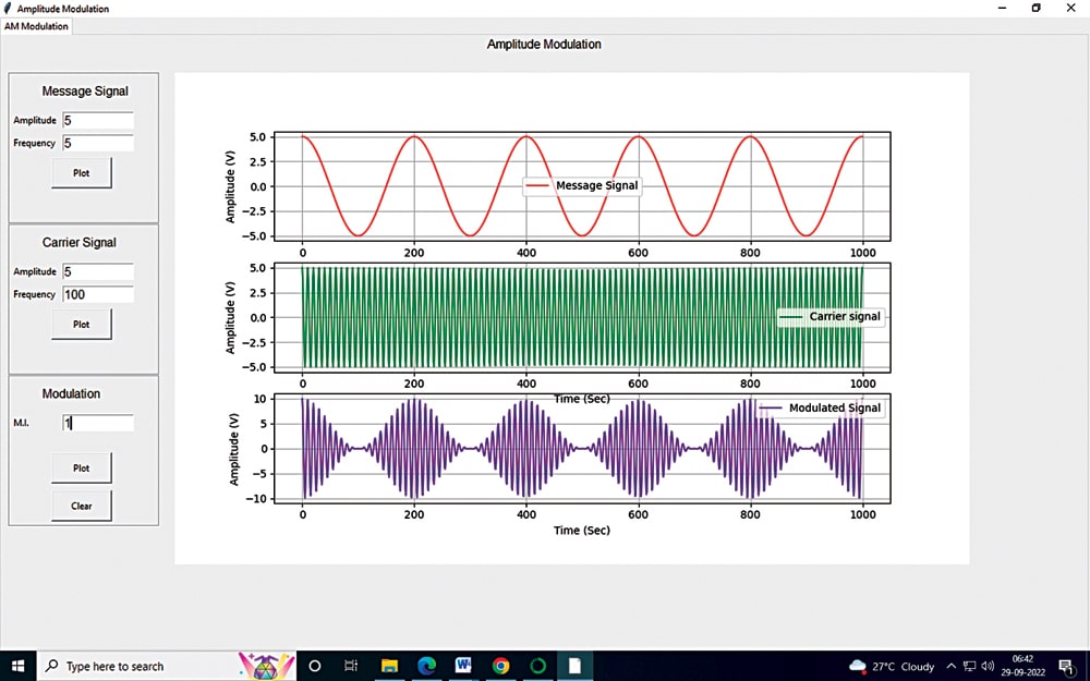
Next, create the graphical user interface (GUI) for the simulator. The GUI includes a window with canvas to plot graphs and entry boxes to get user data for amplitude, frequency of message signal and carrier signals, and for modulation index. It includes three buttons to plot the message signal, career signal, and modulated signal, and for clearing the canvas (see Fig. 4).
Code
In the code, first import various packages of Python for the smooth operation of various functions, as follows:
from tkinter import *
from matplotlib.figure import Figure
from matplotlib.backends.backend_tkagg
import (FigureCanvasTkAgg, Navigation
Toolbar2Tk)
from tkinter import ttk
import numpy as np
To display root window and manage other components in this window, use Tk() function for first displaying the root window. The event loop of this window is created by mainloop() function. The title of root window can be provided here. The following coding snippet shows this procedure:
root = Tk()
root.title(‘Amplitude Modulation’)
fig1 = Figure(figsize=(2, 2), dpi=100)
An interface between the Figure and Tkinter Canvas is provided by the FigureCanvasTkAgg class. Here, you may design a canvas of width=1050 and height=650 by positioning it at x=230, y=50, as follows:
canvas = FigureCanvasTkAgg(fig1,
master=tab1)
canvas.draw_idle()
canvas.get_tk_widget().place(x=230, y=50,
width=1050, height=650)
Next, create the widgets for plotting the message, career, and modulated signals. For user-defined values of amplitude and frequency of the signal, use the entry widget from the Tkinter package. These values are stored in variables for further calculation. All widgets are grouped by using the frame function.
Two button widgets are used for plotting the message and carrier signals. The commands for these buttons are defined by taking inputs from entry widget variables (Amplitude and Frequency) and using the sin function from the NumPy package of Python.
The mathematical equation for the modulated signal is defined in Eq 3. This is plotted by using the NumPy package. The user-defined modulation index is used for calculating and plotting the modulated signal.
A button for clearing the plotting in canvas needs to be designed. This can be achieved by the .clear() function.
To test, run the simulator code and put the values for signal modulation. Test perfect modulation under Modulation and over modulation of signals using the simulation. The testing cases are shown as follows.
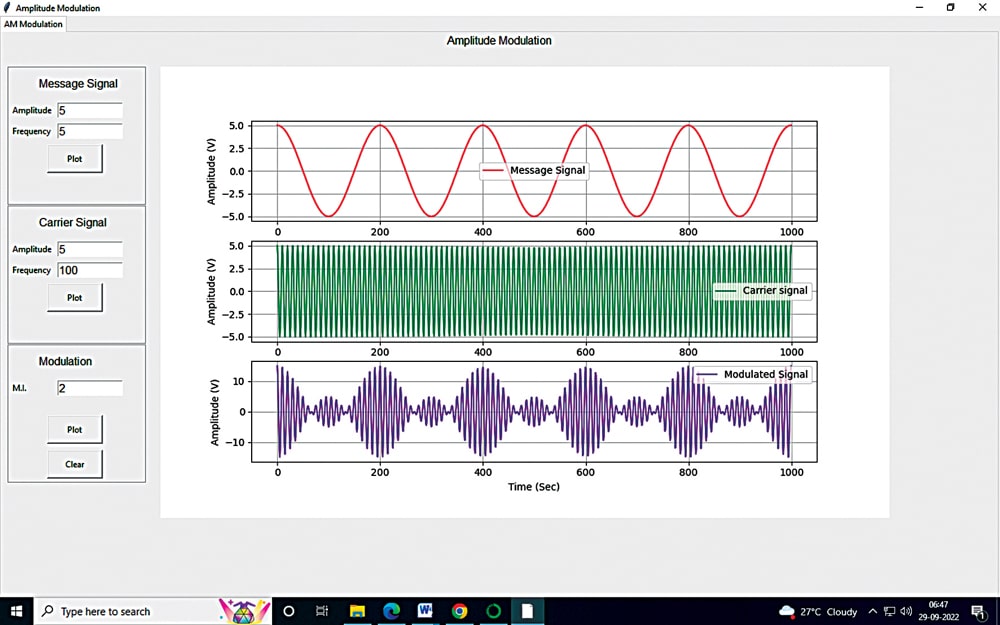
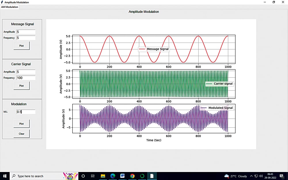
When the modulation index is maintained at value 1, as shown in Fig. 5, you get perfect modulation. When the modulation index is below 1, as shown in Fig. 6, it is called under modulation. When the modulation index is above 1, as in Fig. 7, you get over-modulation.
Download source code
Akhtar Nadaf is an electronics enthusiast working at N.K. Orchid College of Engineering and Technology, Solapur