


 This article explains spectrogram of the speech signal (analysis and processing) with MATLAB to get its frequency-domain representation.
In real life, we come across many signals that are variations of the form ƒ(t), where ‘t’ is independent variable ‘time’ in most cases. Temperature, pressure, pulse rate, etc can be plotted along the time axis to see variations across time.
In signal processing, signals can be classified broadly into deterministic signals and stochastic signals. Deterministic signals can be expressed in the form of a mathematical equation and there is no randomness associated with them. The value of the signal at any point of time can be obtained by evaluating the mathematical equation. An example is a pure sine wave:

ƒ(t)=A sin 2πƒt
where ‘A’ is signal amplitude, ‘ƒ’ is signal frequency and ‘t’ is time.

Many of the information-bearing signals may not be predictable in advance. There is a certain amount of randomness in the signal with respect to time. Such signals cannot be expressed in the form of simple mathematical equations. For example, in the noise signal inside a running automobile, we may hear many sounds, including the engine sound, sound of horns from other vehicles and passengers talking, in a combined form with no predictability. Such signals are examples of stochastic signals.
In the speech signal produced when you utter steady sounds like ‘a,’ ‘i’ or ‘u,’ the waveform is a near-periodic repetition of some well-defined patterns. When you produce sounds like ‘s’ and ‘sh,’ the waveform is noise-like. The periodicity in the speech signal is due to the vibration of vocal folds at a particular frequency, known as pitch or fundamental frequency of the speaker. Steady sounds (a, i or u) are examples of vowels and noise-like sounds (s and sh) are examples of consonants. Human speech signal is a chain of vowels and consonants grouped in different forms.
Most of the signals in real life are available continuously and may assume any amplitude value. These signals are called analogue signals and they are not in a form suitable for storing or processing using a digital computer. In digital signal processing, we process the signal as an array of numbers. We do sampling along the time axis to discretise the independent variable ‘t.’ In other words, we look at the signal at a number of time instances separated by a fixed interval ‘T’ (called sampling period==1/ƒs, where ‘ƒs’ is called sampling frequency). Signal values observed at these time instances are further discretised in the amplitude domain to make these suitable for storage in the form of binary digits. This process is called quantisation. After sampling and quantisation (called digitisation) of an analogue signal, the signal assumes the form:
ƒ(n)=qn
where ‘qn’ is an approximation to the signal amplitude at time instant t=nT. The signals so produced are called digital signals. These can be stored in memory and used for processing by mathematical operations with the help of digital computers.
A pure sine-wave after digitisation can be represented as an array in the form:
ƒ(n)=A sin 2πƒnT=A sin 2πƒn/ƒs
where ‘A’ is the signal amplitude, ‘ƒ’ is the signal frequency, ‘ƒs’ is the sampling frequency and ‘n’ is an integer called time index. Sample value (n) is an approximation of the signal amplitude at time instant t=nT.
Understanding the speech signal
Record vowel sound ‘aa’ using the computer’s microphone and save it as a wav file. Select sampling frequency as 10kHz. You may use audio processing software like Praat, Audacity, Goldwave or Wavesurfer to record the signal in wav format at the required sampling frequency.
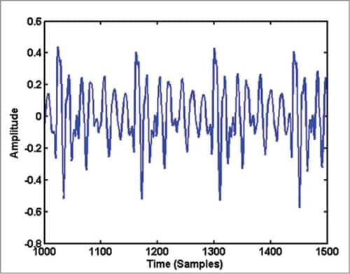
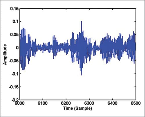
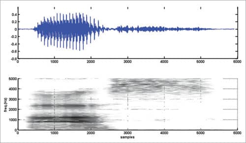
The waveform of the signal, which is a plot of the amplitude of the speech signal for each sample instant, looks like Fig. 1. The horizontal axis is time units in samples and the vertical axis is amplitude of the corresponding samples. If you record sound ‘as’ in which consonant sound ‘s’ follows the vowel sound ‘a,’ and plot the signal, the waveform may look like Fig. 2.
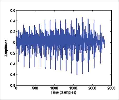

On close examination of Fig. 1, you can see some repeating pattern in it. A zoomed version of Fig. 1 showing samples in the range 1000 to 1500 is given in Fig. 3. If you plot samples from 6000 to 6500 in Fig. 2, you get Fig. 4. Obviously, the waveform in Fig. 4 has no periodicity and it appears noise-like. In the waveform of vowel-consonant sound ‘as,’ you can see that the speech signal properties transform gradually from a nearly periodic signal (samples 2000 to 5000) to a noise-like signal (samples 5000 to 10000).
Frequency-domain analysis of the speech signal
Waveform is a representation of the speech signal. It is a visualisation of the signal in time domain. This representation is almost silent on the frequency contents and the frequency distribution of energy in the speech signal. To get a frequency-domain representation, you need to take Fourier transform of the speech signal. Since speech signal has time-varying properties, the transformation from time-domain to frequency-domain also needs to be done in a time-dependent manner. In other words, you need to take small frames at different points along the time axis, take Fourier transform of the short-duration frames, and then proceed along the time axis towards the end of the utterance. The process is called short-time Fourier transform (STFT). Steps involved in STFT computation are:
1. Select a short-duration frame of the speech signal by windowing
2. Compute Fourier transform of the selected duration
3. Shift the window along the time axis to select the neighbouring frame
4. Repeat step 2 until you reach the end of the speech signal
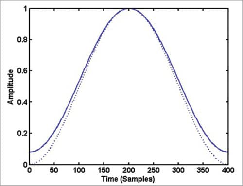
To select a short-duration frame of speech, normally a window function with gradually rising and falling property is used. Commonly used window functions in speech processing are Hamming and Hanning windows. A Hamming window with ‘N’ points is mathematically represented by:
hm(n)=0.54–0.46cos(2πn/N), 0≤n<N
and a Hanning window with ‘N’ points is mathematically represented by:
hn(n)=0.5[1–cos (2πn/N)], 0≤n<N
A window function has non-zero values over a selected set of points and zero values outside this interval. When you multiply a signal with a window function, you get a set of ‘N’ selected samples from the location where you place the window and zero-valued samples at all other points. Fig. 5 shows Hamming and Hanning windows of 400 points each.
You need to finalise the following parameters before computing short-time Fourier transform of the speech signal:
1. Type of window function to be used for framing the speech signal
2. Frame length Nwt in milliseconds
3. Frame shift Nst in milliseconds
4. DFT length
For a sampling frequency of ƒs, you have to use:
Nw=Nwt ƒs /1000
Ns=Nst ƒs /1000
to convert the frame length and frame shift (Nwt, Nst) in milliseconds into the corresponding number in samples (Nwt, Nst). Here fs is the sampling frequency of the speech signal expressed in Hertz. Once these parameters are finalised, framing operation is performed using the MATLAB user-defined function (needs to be copied to the same folder where the main program is stored):
frames = speech2frames( speech, Nw, Ns,
‘cols’, hanning, false );
Generally, frame-duration parameter Nwt and frame-shift parameter Nst are selected such that consecutive frames have sufficient overlap.The condition Nst<Nwt ensures an overlapping window placement. In speech processing applications, overlapping is generally kept above percent by proper selection of Nst and Nwt. The framing operation returns a number of short-duration frames selected using the window function with the specified frame length and frameshift parameters. Each frame is stored as a column vector in the returned array. Once the framing is performed, DFT operation is used to transform each frame to a frequency domain using the command:
MAG = abs( fft(frames,nfft,1) );
Parameter ‘nfft’ specifies the number of points in the DFT operation. It is kept as a power of 2 and must be greater than the frame length in samples. Assuming the wav file has sampling frequency fs of 10kHz, we have used 1024 points as ‘nfft’ for a frame length of 400 samples (40ms). If the sampling frequency of the wav file is not 10kHz, the file needs to be resampled to 10kHz for proper working of the program.Frame shift parameter is set as 100 samples (10ms). MAG variable has the absolute value of Fourier transform of frames stored column wise. The magnitude of Fourier transform is also called spectrum of that frame of the signal. As the speech signal has time-varying properties, the spectrum also goes on varying with time as we move along the samples in the wav file.
Magnitude spectrum computed for individual frames can be represented in many forms. We have been following three parameters: Frame number (indicator of the time axis), DFT bin number (indicator of the frequency axis) and magnitude of DFT computed (indicator of the spectral energy).
These three parameters can be represented conveniently in a 2D format using spectrogram. Spectrogram can be considered as an image representing time and frequency parameters (along X and Y axes) and magnitude values as the intensity of pixels in the X-Y plane. Stronger magnitudes get represented by dark spots and silences (low- or zero-amplitude signals) get represented by white spots in the image.
For a real valued signal, you need to take only the first half of the magnitude spectrum, since the spectrum has a symmetric shape with respect to nfft/2. You will see that the range of values in the computed magnitude spectrum is very high as you move from frames with valid speech signal to frames involving silences or pauses. It is better to limit the dynamic range to a fixed value before plotting. The magnitude spectrum is converted into the log scale and its dynamic range is limited to 50dB in the main program (spectrogram_efy.m) that computes and plots the spectrogram of a speech signal.
Parameters Nwt and Nst decide the resolving power of the spectrogram along time and frequency axes. Spectrograms obtained with Nwt values greater than 20ms are called narrowband spectrograms. Generally, these have a good frequency resolution. Frequency tracks appear as horizontal lines varying in intensity.
When you lower the frame-duration parameter, you need to lower the frame-shift parameter also to avoid missing frames. A reduced value of frame duration results in a lower frequency resolution but a good time resolution. The spectrogram obtained with good time resolution and poor frequency resolution is called a wideband spectrogram. Narrowband spectrograms are useful for accurate frequency analysis of speech signals.

Wideband spectrograms are useful for accurate localisation of transient region onsets in the speech signal.
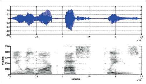
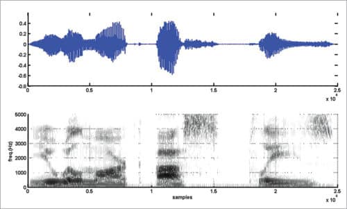
Narrowband and wideband spectrograms for vowel-consonant sound ‘as’ are shown in Figs 6 and 7, respectively. Spectrograms (narrowband and wideband) for the sentence “You will mark as please” are shown in Figs 8 and 9, respectively. Readers are advised to experiment with different speech utterances and different values for Nwt, Nst, and nfft and to observe variations in spectrograms.
Download Source Folder
Check more such MATLAB projects.


Please, how do i calculate MSE and SNR of ECG signal before and after noise?
I need the result for about 300 sample frequencies.
Thank you
Please share MATLAB code to make binaural beats