

If information is the same but its position changes in the next frame, it will not get encoded once again as it was already coded in the firstframe. For example, if the same paperweight is now shifted towards right, its position with respect to macro blocks changes. But it carries the same information as before. So now the motion vector is applied to these particular macro blocks. It will appear with its changed position, but it requires fewer bits for coding the same and hence the reduction in bandwidth.
The predicted frame (frame obtained by applying motion) is then subtracted from the second frame to produce the difference-frame. Both components (motion vector and frame difference) are combined to form a predicted frame (P-frame).

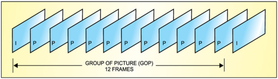
Temporal compression is carried out on a group of pictures normally composed of twelve non-interlaced frames. The firstframe of the group acts as the anchor or reference frame known as the inter-frame (I-frame). This is followed by a P-frame obtained by comparing the second frame with the I-frame. This is then repeated and the third frame is compared with the previous P-frame to produce a second P-frame and so on. This goes on until the end of the group of twelve frames. A new reference I-frame is then inserted for the next group of twelve frames and so on. This type of prediction is known as forward prediction.
Motion vector. Motion vector is obtained by the process of block matching. Y component of the reference frame is divided into 16×16 macro blocks. Blocks are taken one by one and the matching block searched within the given area.
When a match is found, the displacement is used to obtain a motion-compensation vector that describes the movement of the macro block in terms of speed and direction. Only a relatively small amount of data is necessary to describe a motion-compensation vector. The actual pixel values of the macro block do not have to be retransmitted.
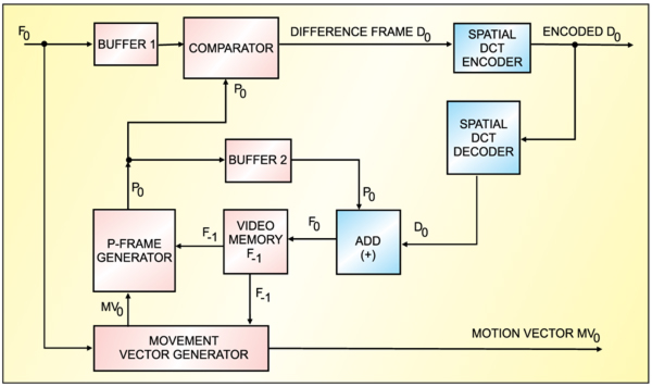
Predicted and difference frames. As shown in Fig. 5, current frame F0 is fed into Buffer-1 and held there for a while. It is also fed into the movement vector generator, which uses the contents of the previous frame F-1 stored in the video memory to obtain motion vector MV0. The motion vector is then added to F-1 to produce pre-dicted frame P0. P0 is compared with the contents of the current frame F0 in Buffer-2 to produce residual error or difference frame D0. Residual error D0 is fed into the spatial discrete cosine transform (DCT) encoder and sent out for transmission.
Encoded D0 is decoded to reproduce D0 as it would be required at the receiving end. D0 is then added to P0, which has been waiting in Buffer-2 to reconstruct current frame F0 for storage in the video memory for the next frame and so on.
Spatial compression
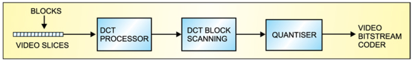
The heart of spatial redundancy removal is the DCT processor. The DCT processor receives video slices in the form of a stream of 8×8 blocks. The blocks may be part of a luminance frame (Y) or a chrominance frame. Sample values representing the pixel of each block are then fed into the DCT processor, which translates them into an 8×8 matrix of DCT coeffiients representing the spatial frequency content of the block. The coefficient are then scanned and quantised before transmission.
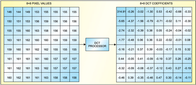
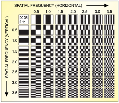
Discrete cosine transform. DCT is used in several coding standards (MPEG 1, MPEG 2, H.263, etc) to remove spatial redundancy that exists between neighbouring pixels in a image. It is a Fourier transform which takes information in the time domain and expresses it in the frequency domain. Normal pictures are two-dimensional and contain diagonal as well as horizontal and vertical spatial frequencies. MPEG-2 specifies DCT as the method of transforming spatial picture information into spatial frequency components. Each spatial frequency is given a value known as the DCT coefficient.For an 8×8 block of pixel samples, an 8×8 block of DCT coefficients is produced (refe Fig. 7).
A block that contains different picture details is represented by various coefficient values in the appropriate cells. Coarse picture details utilise a number of cells towards the left top corner, and the cells and finepicture details utilise a number of cells towards the bottom right-hand corner.
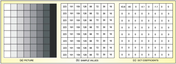
The grey-scale pattern is shown in Fig. 9(a). The corresponding sample values are shown in Fig. 9(b) and DCT coefficients in Fig. 9(c). DCT does not directly reduce the number of bits required to represent the 8×8-pixel block. Sixty-four pixel sample values are replaced with 64 DCT coefficient values
The reduction in the number of bits follows from the fact that for a typical block of a natural image, the distribution of the DCT coefficiens is not uniform. An average DCT matrix has most of its coeffiients—and therefore energy—concentrated at and around the top left-hand corner. The bottom right-hand quadrant has very few coefficiens of any substantial value. Bit rate reduction may thus be achieved by not transmitting the zero and near-zero coefficients Further bit reduction may be introduced by weighted quantising and special coding techniques of the remaining coefficients.
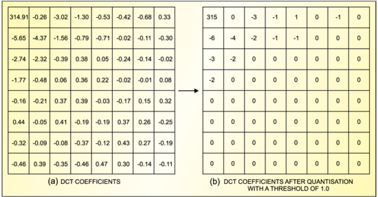
Quantising the DCT block. After a block has been transformed, the DCT coefficients are quantised (rounded u or down) to a smaller set of possible values to produce a simplified set of coefficients.
The DCT block (shown in Fig. 10(a)) may be reduced to very few coefficients (Fig. 10(b)) if a threshold of 1.0 is applied. After this, a non-linear or weighted quantisation is applied. The video samples are given a linear quantisation but the DCT coefficient receive a non-linear quantisation. A different quantisation level is applied to each coefficient depending on the spatial frequency it represents within the block.
High quantisation levels are allocated to coefficients representing low spatial frequencies. This is because the human eye is the most sensitive to low spatial frequencies. Lower quantisation is applied to coefficients representing high spatial frequencies. This increases quantisation error at these high frequencies, introducing error noise that is irreversible at the receiver. However, these errors are tolerable since high-frequency noise is less visible than low-frequency noise.
The DCT coefficient at the top left-hand is treated as a special case and given the highest priority. A more effective weighted quantisation may be applied to the chrominance frames since quantisation error is less visible in the chrominance component than in the luminance component. Quantisation error is more visible in some blocks than in others. One place where it shows up is blocks that contain a high contrast edge between two plain areas. The quantisation parameters can be modified to limit the quantisation error, particularly in high-frequency cells.
Daniel A. Figueiredo is scientist-D, and Sidhant Kulkarni and Umesh Shirale are pursuing M.Tech in electronics design and technology at DOEACC centre, Aurangabad